Week 9 Wednesday

Comment: The attached file mnist.csv contains 42,000 of the usual 70,000 handwritten digits. I decreased the number of rows just to make it a smaller size for uploading to Deepnote; even this smaller version is 73 megabytes. (I wouldn’t have done this if I were working locally on my own computer.)

import pandas as pd
import numpy as np
import matplotlib.pyplot as plt
import altair as alt
alt.data_transformers.enable('default', max_rows = 10000)

from sklearn.datasets import make_regression

Part 1 - PCA with simulated data

X, y, m = make_regression(n_samples=4000, n_features=1, noise=20, coef=True, random_state=529)
df = pd.DataFrame(X, columns=["x"])
df["y"] = y

alt.Chart(df).mark_circle().encode(
    x="x",
    y="y"
)

from sklearn.decomposition import PCA

pca_model = PCA()

# Just input, no target, since unsupervised
pca_model.fit(df)

PCA()

In a Jupyter environment, please rerun this cell to show the HTML representation or trust the notebook.
On GitHub, the HTML representation is unable to render, please try loading this page with nbviewer.org.

arr = pca_model.transform(df)

type(arr)

numpy.ndarray

arr[:3]

array([[-11.9795057 ,   0.41887263],
       [  2.54206288,  -0.20554913],
       [-32.28415112,  -0.39903818]])

df_transform = pd.DataFrame(arr, columns=["PC1", "PC2"])

alt.Chart(df_transform).mark_circle().encode(
    x="PC1",
    y="PC2"
)

alt.Chart(df_transform).mark_circle().encode(
    x="PC1",
    y=alt.Y("PC2", scale=alt.Scale(domain=(-150, 150)))
)

pca_model.explained_variance_ratio_

array([9.99780409e-01, 2.19591117e-04])

Part 2 - PCA with MNIST

df = pd.read_csv("mnist.csv")

df[:3]

	label	pixel0	pixel1	pixel2	pixel3	pixel4	pixel5	pixel6	pixel7	pixel8	...	pixel774	pixel775	pixel776	pixel777	pixel778	pixel779	pixel780	pixel781	pixel782	pixel783
0	1	0	0	0	0	0	0	0	0	0	...	0	0	0	0	0	0	0	0	0	0
1	0	0	0	0	0	0	0	0	0	0	...	0	0	0	0	0	0	0	0	0	0
2	1	0	0	0	0	0	0	0	0	0	...	0	0	0	0	0	0	0	0	0	0

3 rows × 785 columns

df_label = df["label"]

df_X = df.loc[:, "pixel0":]

df_X.shape

(42000, 784)

fig, ax = plt.subplots()
ax.imshow(df_X.iloc[178].to_numpy().reshape((28,28)), cmap="binary");

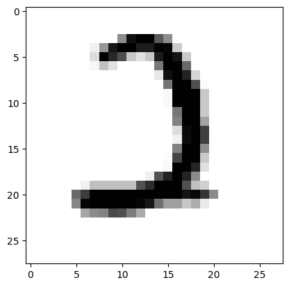
df_label.iloc[178]

2

Restrict the dataset to only images of 0 and 8.

bool_ser = df_label.isin([0,8])
bool_ser

0        False
1         True
2        False
3        False
4         True
         ...  
41995     True
41996    False
41997    False
41998    False
41999    False
Name: label, Length: 42000, dtype: bool

X_sub = df_X[bool_ser]
y_sub = df_label[bool_ser]

y_sub.value_counts()

label
0    4132
8    4063
Name: count, dtype: int64

X_sub.shape

(8195, 784)

pca = PCA(n_components=2)

pca.fit(X_sub)

PCA(n_components=2)

In a Jupyter environment, please rerun this cell to show the HTML representation or trust the notebook.
On GitHub, the HTML representation is unable to render, please try loading this page with nbviewer.org.

X_transform = pca.transform(X_sub)

df_transform = pd.DataFrame(X_transform, columns=["PC1", "PC2"])

df_transform[:3]

	PC1	PC2
0	1160.227253	-1048.161600
1	1514.001737	-1096.474230
2	-45.408654	-45.805242

alt.Chart(df_transform).mark_circle().encode(
    x="PC1",
    y="PC2"
)

df_transform[:3]

	PC1	PC2
0	1160.227253	-1048.161600
1	1514.001737	-1096.474230
2	-45.408654	-45.805242

y_sub[:3]

1    0
4    0
5    0
Name: label, dtype: int64

y_sub.reset_index(drop=True)

0       0
1       0
2       0
3       8
4       0
       ..
8190    0
8191    8
8192    0
8193    0
8194    0
Name: label, Length: 8195, dtype: int64

df_transform["label"] = y_sub.reset_index(drop=True)

df_transform[:3]

	PC1	PC2	label
0	1160.227253	-1048.161600	0
1	1514.001737	-1096.474230	0
2	-45.408654	-45.805242	0

alt.Chart(df_transform).mark_circle().encode(
    x="PC1",
    y="PC2",
    color="label:N"
)

df_reset = df_transform.reset_index()
df_reset

	index	PC1	PC2	label
0	0	1160.227253	-1048.161600	0
1	1	1514.001737	-1096.474230	0
2	2	-45.408654	-45.805242	0
3	3	-553.621756	785.414302	8
4	4	779.665844	1178.590268	0
...	...	...	...	...
8190	8190	1446.677423	529.649470	0
8191	8191	-764.906679	-595.978439	8
8192	8192	905.435172	381.444734	0
8193	8193	919.788642	-495.668776	0
8194	8194	744.664272	-520.716016	0

8195 rows × 4 columns

alt.Chart(df_reset).mark_circle().encode(
    x="PC1",
    y="PC2",
    color="label:N",
    tooltip="index"
)

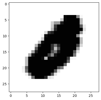
arr_outlier = X_sub.iloc[7663].to_numpy().reshape((28,28))

fig, ax = plt.subplots()
ax.imshow(arr_outlier, cmap="binary")

<matplotlib.image.AxesImage at 0x7ff02a20ecd0>

Created in Deepnote