PyTorch and Neural Networks
PyTorch and Neural Networks
YuJa video from lecture
from tqdm.std import tqdm, trange
from tqdm import notebook
notebook.tqdm = tqdm
notebook.trange = trange

import pandas as pd
import numpy as np
import matplotlib.pyplot as plt

import torch
from torch import nn
from torchvision import datasets
from torchvision.transforms import ToTensor
from torch.utils.data import DataLoader
The first four lines
from tqdm.std import tqdm, trange
from tqdm import notebook
notebook.tqdm = tqdm
notebook.trange = trange
are an ad hoc suggestion I read on a Deepnote forum to help prevent a minor error (the error is just because of a progress bar, nothing important). Don’t worry about them.
# Load the data
training_data = datasets.MNIST(
    root="data",
    train=True,
    download=True,
    transform=ToTensor(),
)

test_data = datasets.MNIST(
    root="data",
    train=False,
    download=True,
    transform=ToTensor(),
)
YouTube video on Neural Networks from 3Blue1Brown. Recommended clips:
2:42-5:30
8:40-12:40
training_data.data.shape
torch.Size([60000, 28, 28])
training_data.data[13]
tensor([[  0,   0,   0,   0,   0,   0,   0,   0,   0,   0,   0,   0,   0,   0,
           0,   0,   0,   0,   0,   0,   0,   0,   0,   0,   0,   0,   0,   0],
        [  0,   0,   0,   0,   0,   0,   0,   0,   0,   0,   0,   0,   0,   0,
           0,   0,   0,   0,   0,   0,   0,   0,   0,   0,   0,   0,   0,   0],
        [  0,   0,   0,   0,   0,   0,   0,   0,   0,   0,   0,   0,   0,   0,
           0,   0,  38, 222, 225,   0,   0,   0,   0,   0,   0,   0,   0,   0],
        [  0,   0,   0,   0,   0,   0,   0,   0,   0,   0,   0,   0,   0,   0,
           0, 147, 234, 252, 176,   0,   0,   0,   0,   0,   0,   0,   0,   0],
        [  0,   0,   0,   0,   0,   0,   0,   0,   0,   0,   0,   0,   0,  23,
         197, 253, 252, 208,  19,   0,   0,   0,   0,   0,   0,   0,   0,   0],
        [  0,   0,   0,   0,   0,   0,   0,   0,   0,   0,   0,   0,  38, 178,
         252, 253, 117,  65,   0,   0,   0,   0,   0,   0,   0,   0,   0,   0],
        [  0,   0,   0,   0,   0,   0,   0,   0,   0,   0,   0,   0,  57, 252,
         252, 253,  89,   0,   0,   0,   0,   0,   0,   0,   0,   0,   0,   0],
        [  0,   0,   0,   0,   0,   0,   0,   0,   0,   0,   0,  38, 222, 253,
         253,  79,   0,   0,   0,   0,   0,   0,   0,   0,   0,   0,   0,   0],
        [  0,   0,   0,   0,   0,   0,   0,   0,   0,   0,   0, 131, 252, 179,
          27,   0,   0,   0,   0,   0,   0,   0,   0,   0,   0,   0,   0,   0],
        [  0,   0,   0,   0,   0,   0,   0,   0,   0,   0, 198, 246, 220,  37,
           0,   0,   0,   0,   0,   0,   0,   0,   0,   0,   0,   0,   0,   0],
        [  0,   0,   0,   0,   0,   0,   0,   0,   0,  79, 253, 252, 135,  28,
           0,   0,   0,   0,   0,   0,   0,   0,   0,   0,   0,   0,   0,   0],
        [  0,   0,   0,   0,   0,   0,   0,   0,  16, 140, 253, 252, 118,   0,
           0,   0,   0, 111, 140, 140,   0,   0,   0,   0,   0,   0,   0,   0],
        [  0,   0,   0,   0,   0,   0,   0,   0,  13, 191, 255, 253,  56,   0,
           0, 114, 113, 222, 253, 253, 255,  27,   0,   0,   0,   0,   0,   0],
        [  0,   0,   0,   0,   0,   0,   0,   0,  76, 252, 253, 223,  37,   0,
          48, 174, 252, 252, 242, 214, 253, 199,  31,   0,   0,   0,   0,   0],
        [  0,   0,   0,   0,   0,   0,   0,  13, 109, 252, 228, 130,   0,  38,
         165, 253, 233, 164,  49,  63, 253, 214,  31,   0,   0,   0,   0,   0],
        [  0,   0,   0,   0,   0,   0,   0,  73, 252, 252, 126,   0,  23, 178,
         252, 240, 148,   7,  44, 215, 240, 148,   0,   0,   0,   0,   0,   0],
        [  0,   0,   0,   0,   0,   0,   0, 119, 252, 252,   0,   0, 197, 252,
         252,  63,   0,  57, 252, 252, 140,   0,   0,   0,   0,   0,   0,   0],
        [  0,   0,   0,   0,   0,   0,   0, 135, 253, 174,   0,  48, 229, 253,
         112,   0,  38, 222, 253, 112,   0,   0,   0,   0,   0,   0,   0,   0],
        [  0,   0,   0,   0,   0,   0,   0, 135, 252, 173,   0,  48, 227, 252,
         158, 226, 234, 201,  27,  12,   0,   0,   0,   0,   0,   0,   0,   0],
        [  0,   0,   0,   0,   0,   0,   0,  57, 252, 252,  57, 104, 240, 252,
         252, 253, 233,  74,   0,   0,   0,   0,   0,   0,   0,   0,   0,   0],
        [  0,   0,   0,   0,   0,   0,   0,  51, 242, 252, 253, 252, 252, 252,
         252, 240, 148,   0,   0,   0,   0,   0,   0,   0,   0,   0,   0,   0],
        [  0,   0,   0,   0,   0,   0,   0,   0,  75, 189, 253, 252, 252, 157,
         112,  63,   0,   0,   0,   0,   0,   0,   0,   0,   0,   0,   0,   0],
        [  0,   0,   0,   0,   0,   0,   0,   0,   0,   0,   0,   0,   0,   0,
           0,   0,   0,   0,   0,   0,   0,   0,   0,   0,   0,   0,   0,   0],
        [  0,   0,   0,   0,   0,   0,   0,   0,   0,   0,   0,   0,   0,   0,
           0,   0,   0,   0,   0,   0,   0,   0,   0,   0,   0,   0,   0,   0],
        [  0,   0,   0,   0,   0,   0,   0,   0,   0,   0,   0,   0,   0,   0,
           0,   0,   0,   0,   0,   0,   0,   0,   0,   0,   0,   0,   0,   0],
        [  0,   0,   0,   0,   0,   0,   0,   0,   0,   0,   0,   0,   0,   0,
           0,   0,   0,   0,   0,   0,   0,   0,   0,   0,   0,   0,   0,   0],
        [  0,   0,   0,   0,   0,   0,   0,   0,   0,   0,   0,   0,   0,   0,
           0,   0,   0,   0,   0,   0,   0,   0,   0,   0,   0,   0,   0,   0],
        [  0,   0,   0,   0,   0,   0,   0,   0,   0,   0,   0,   0,   0,   0,
           0,   0,   0,   0,   0,   0,   0,   0,   0,   0,   0,   0,   0,   0]],
       dtype=torch.uint8)
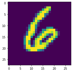
Using the default color map.
fig, ax = plt.subplots()
ax.imshow(training_data.data[13])
<matplotlib.image.AxesImage at 0x7fe43261a490>

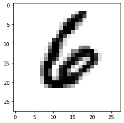
Using the binary color map.
fig, ax = plt.subplots()
ax.imshow(training_data.data[13],cmap='binary')
<matplotlib.image.AxesImage at 0x7fe432e41c70>

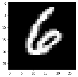
Switching to the reversed color map, by appending _r to the end of the cmap name.
fig, ax = plt.subplots()
ax.imshow(training_data.data[13],cmap='binary_r')
<matplotlib.image.AxesImage at 0x7fe40054d790>

That should correspond to the number 6.
training_data.targets[13]
tensor(6)
To convert a length-one PyTorch tensor to a single number, we use .item().
training_data.targets[13].item()
6
In the 3Blue1Brown video, the grid of image pixels gets “flattened” out into a length 784 vector. PyTorch has a standard way of doing this, using nn.Flatten().
flatten = nn.Flatten()
flatten(training_data.data[:13])
tensor([[0, 0, 0,  ..., 0, 0, 0],
        [0, 0, 0,  ..., 0, 0, 0],
        [0, 0, 0,  ..., 0, 0, 0],
        ...,
        [0, 0, 0,  ..., 0, 0, 0],
        [0, 0, 0,  ..., 0, 0, 0],
        [0, 0, 0,  ..., 0, 0, 0]], dtype=torch.uint8)
training_data.data[:13].shape
torch.Size([13, 28, 28])
flatten(training_data.data[:13]).shape
torch.Size([13, 784])
PyTorch uses many elements of Object Oriented programming. In the following, we are defining a new type of object called ThreeBlue. You don’t need to understand all of the details; we will try to make clear what you should understand and what is less important for us, for example, in the class Learning Objectives.
The name __init__ defined below begins and ends with two underscores. These sorts of methods are called dunder methods for double underscore. They lie in the background of many Python operations. For example, when you add two objects together, that is often (always?) secretly using the __add__ dunder method. The __init__ method is a method that is called when a new object is created of this class.
The class ThreeBlue below is the beginning of a tiny neural network.
class ThreeBlue(nn.Module):
    def __init__(self):
        super().__init__()
        self.flatten = nn.Flatten()

    def forward(self,x):
        y = self.flatten(x)
        return y
mon = ThreeBlue()
I don’t totally understand what the __main__ means in the following; the important part is that the object mon we have instantiated is of type ThreeBlue.
type(mon)
__main__.ThreeBlue
We defined a flatten attribute in the __init__ method above, so that is why mon has a flatten attribute. We can use it just like the flatten above.
mon.flatten
Flatten(start_dim=1, end_dim=-1)
mon.flatten(training_data.data[:13])
tensor([[0, 0, 0,  ..., 0, 0, 0],
        [0, 0, 0,  ..., 0, 0, 0],
        [0, 0, 0,  ..., 0, 0, 0],
        ...,
        [0, 0, 0,  ..., 0, 0, 0],
        [0, 0, 0,  ..., 0, 0, 0],
        [0, 0, 0,  ..., 0, 0, 0]], dtype=torch.uint8)
Here is a slightly bigger neural network.
class ThreeBlue(nn.Module):
    def __init__(self):
        super().__init__()
        self.flatten = nn.Flatten()
        self.layers = nn.Sequential(
            nn.Linear(784,10)
        )

    def forward(self,x):
        y = self.flatten(x)
        z = self.layers(y)
        return z
mon = ThreeBlue()
The entries in training_data.data are integers between 0 and 255. We want floats instead, and numbers between 0 and 1 is more natural anyway, so we can fix the following error by dividing by 255. This can also be accomplished using the ToTensor function that is written above (we will see it later).
mon(training_data.data)
---------------------------------------------------------------------------
RuntimeError                              Traceback (most recent call last)
Input In [21], in <module>
----> 1 mon(training_data.data)

File ~/miniconda3/envs/torch/lib/python3.8/site-packages/torch/nn/modules/module.py:1102, in Module._call_impl(self, *input, **kwargs)
   1098 # If we don't have any hooks, we want to skip the rest of the logic in
   1099 # this function, and just call forward.
   1100 if not (self._backward_hooks or self._forward_hooks or self._forward_pre_hooks or _global_backward_hooks
   1101         or _global_forward_hooks or _global_forward_pre_hooks):
-> 1102     return forward_call(*input, **kwargs)
   1103 # Do not call functions when jit is used
   1104 full_backward_hooks, non_full_backward_hooks = [], []

Input In [19], in ThreeBlue.forward(self, x)
      9 def forward(self,x):
     10     y = self.flatten(x)
---> 11     z = self.layers(y)
     12     return z

File ~/miniconda3/envs/torch/lib/python3.8/site-packages/torch/nn/modules/module.py:1102, in Module._call_impl(self, *input, **kwargs)
   1098 # If we don't have any hooks, we want to skip the rest of the logic in
   1099 # this function, and just call forward.
   1100 if not (self._backward_hooks or self._forward_hooks or self._forward_pre_hooks or _global_backward_hooks
   1101         or _global_forward_hooks or _global_forward_pre_hooks):
-> 1102     return forward_call(*input, **kwargs)
   1103 # Do not call functions when jit is used
   1104 full_backward_hooks, non_full_backward_hooks = [], []

File ~/miniconda3/envs/torch/lib/python3.8/site-packages/torch/nn/modules/container.py:141, in Sequential.forward(self, input)
    139 def forward(self, input):
    140     for module in self:
--> 141         input = module(input)
    142     return input

File ~/miniconda3/envs/torch/lib/python3.8/site-packages/torch/nn/modules/module.py:1102, in Module._call_impl(self, *input, **kwargs)
   1098 # If we don't have any hooks, we want to skip the rest of the logic in
   1099 # this function, and just call forward.
   1100 if not (self._backward_hooks or self._forward_hooks or self._forward_pre_hooks or _global_backward_hooks
   1101         or _global_forward_hooks or _global_forward_pre_hooks):
-> 1102     return forward_call(*input, **kwargs)
   1103 # Do not call functions when jit is used
   1104 full_backward_hooks, non_full_backward_hooks = [], []

File ~/miniconda3/envs/torch/lib/python3.8/site-packages/torch/nn/modules/linear.py:103, in Linear.forward(self, input)
    102 def forward(self, input: Tensor) -> Tensor:
--> 103     return F.linear(input, self.weight, self.bias)

File ~/miniconda3/envs/torch/lib/python3.8/site-packages/torch/nn/functional.py:1848, in linear(input, weight, bias)
   1846 if has_torch_function_variadic(input, weight, bias):
   1847     return handle_torch_function(linear, (input, weight, bias), input, weight, bias=bias)
-> 1848 return torch._C._nn.linear(input, weight, bias)

RuntimeError: expected scalar type Float but found Byte
training_data.data.numpy().max()
255
training_data.data.max()
tensor(255, dtype=torch.uint8)
mon(training_data.data/255)
tensor([[-0.2732, -0.3196, -0.1517,  ..., -0.1586, -0.1426,  0.1017],
        [-0.1850, -0.1077, -0.1705,  ..., -0.0937, -0.1251,  0.1382],
        [-0.3156, -0.0272,  0.2463,  ...,  0.0058, -0.0822, -0.0833],
        ...,
        [-0.1902, -0.4926, -0.1165,  ..., -0.1051, -0.0940,  0.2293],
        [-0.2706, -0.0412, -0.0826,  ...,  0.0597,  0.1251, -0.1615],
        [-0.1423, -0.0788, -0.1058,  ..., -0.1499,  0.0773, -0.0987]],
       grad_fn=<AddmmBackward0>)
Notice that we never explicitly call the forward method of mon. PyTorch is calling this for us in the background; we should not call it directly.
Here is the input shape.
training_data.data.shape
torch.Size([60000, 28, 28])
Here is the output shape.
mon(training_data.data/255).shape
torch.Size([60000, 10])
Think of a neural network as a function. For each input data point for MNIST handwritten digits, we want 10 outputs. After rescaling, we can think of these 10 outputs as probabilities for each possible true value of the digit.
In the current version, some of these 10 numbers are negative, so we can’t think of them directly as probabilities.
mon(training_data.data[13:14]/255)
tensor([[-0.2600,  0.1508,  0.0664, -0.0762, -0.0020, -0.0805, -0.3462, -0.2443,
          0.2733, -0.0991]], grad_fn=<AddmmBackward0>)
But we can at least find the index of the largest number, which could be our predicted digit. (Think of dim=1 as analogous to axis=1 from pandas and NumPy.)
mon(training_data.data[13:14]/255).argmax(dim=1)
tensor([8])
Another option is that we could rescale these numbers, using the sigmoid function, then they will at least be between 0 and 1, so they can be interpreted as probabilities. Notice how the original outputs were clustered around 0, and the new outputs are clustered around 0.5.
sigmoid = nn.Sigmoid()
sigmoid(mon(training_data.data[13:14]/255))
tensor([[0.4354, 0.5376, 0.5166, 0.4810, 0.4995, 0.4799, 0.4143, 0.4392, 0.5679,
         0.4752]], grad_fn=<SigmoidBackward0>)
Another option, which we will actually not use very often, is to apply a function called Softmax, which not only scales the numbers into the correct range, but also makes them sum to 1.
softmax = nn.Softmax(dim=1)
softmax(mon(training_data.data[13:14]/255))
tensor([[0.0807, 0.1216, 0.1118, 0.0969, 0.1044, 0.0965, 0.0740, 0.0819, 0.1375,
         0.0947]], grad_fn=<SoftmaxBackward0>)
softmax(mon(training_data.data[13:14]/255)).sum()
tensor(1.0000, grad_fn=<SumBackward0>)
