Subject of Subjectivity: The Global Happiness Index

Subject of Subjectivity: The Global Happiness Index#

Author: Rachel Bronder rbronder@uci.edu Course Project, UC Irvine, Math 10, S23

Introduction#

In this project, I will be analyzing the global Happiness Index for 2018, a dataset I found on Kaggle at https://www.kaggle.com/datasets/sougatapramanick/happiness-index-2018-2019?resource=download&select=2018.csv . The abstract of the dataset mentions that there is a relationship between several independent variables, including “GDP per capita,” “freedom to make life choices,” “health life expectancy,” “perception of corruption,” and “social support”, and the dependent variable of the happiness score. I would like to acknowledge that at the time I am creating this project, which is June 2023, this data is from about 5 years ago. Therefore, some of the rankings may be outdated.

My goal for this project is to see how the factors of the happiness score and happiness ranking relate with one another. Can any connections be made between one column category and another? How does the ranking correlate to any of the particular factors?

Picture title

Taking a look at the data#

Before we do anything with our dataset, lets see what we are working with.

import pandas as pd
import seaborn as sns
import altair as alt

df = pd.read_csv('2018.csv')

df.head()

	Overall rank	Country or region	Score	GDP per capita	Social support	Healthy life expectancy	Freedom to make life choices	Generosity	Perceptions of corruption
0	1	Finland	7.632	1.305	1.592	0.874	0.681	0.202	0.393
1	2	Norway	7.594	1.456	1.582	0.861	0.686	0.286	0.340
2	3	Denmark	7.555	1.351	1.590	0.868	0.683	0.284	0.408
3	4	Iceland	7.495	1.343	1.644	0.914	0.677	0.353	0.138
4	5	Switzerland	7.487	1.420	1.549	0.927	0.660	0.256	0.357

I am cleaning up the data, removing any rows with not-a-number values.

df = df.dropna(axis=0)
df

	Overall rank	Country or region	Score	GDP per capita	Social support	Healthy life expectancy	Freedom to make life choices	Generosity	Perceptions of corruption
0	1	Finland	7.632	1.305	1.592	0.874	0.681	0.202	0.393
1	2	Norway	7.594	1.456	1.582	0.861	0.686	0.286	0.340
2	3	Denmark	7.555	1.351	1.590	0.868	0.683	0.284	0.408
3	4	Iceland	7.495	1.343	1.644	0.914	0.677	0.353	0.138
4	5	Switzerland	7.487	1.420	1.549	0.927	0.660	0.256	0.357
...	...	...	...	...	...	...	...	...	...
151	152	Yemen	3.355	0.442	1.073	0.343	0.244	0.083	0.064
152	153	Tanzania	3.303	0.455	0.991	0.381	0.481	0.270	0.097
153	154	South Sudan	3.254	0.337	0.608	0.177	0.112	0.224	0.106
154	155	Central African Republic	3.083	0.024	0.000	0.010	0.305	0.218	0.038
155	156	Burundi	2.905	0.091	0.627	0.145	0.065	0.149	0.076

156 rows × 9 columns

type(df["Country or region"])

pandas.core.series.Series

df.dtypes

Overall rank                      int64
Country or region                object
Score                           float64
GDP per capita                  float64
Social support                  float64
Healthy life expectancy         float64
Freedom to make life choices    float64
Generosity                      float64
Perceptions of corruption       float64
dtype: object

df.shape

(156, 9)

c1 = alt.Chart(df).mark_bar().encode(
    x = "Country or region",
    y = "Score"
)
c1
#Here we see a bar graph of each country where the bar is raised to the level 
#of it's corresponding happiness score

alt.Chart(df).mark_geoshape().encode(
        color = "Overall rank")

import altair as alt
from vega_datasets import data
import geopandas as gpd

url = "https://naciscdn.org/naturalearth/110m/cultural/ne_110m_admin_0_countries.zip"
gdf_ne = gpd.read_file(url)  # zipped shapefile
gdf_ne = gdf_ne[["NAME", "CONTINENT", "POP_EST", 'geometry']]

alt.Chart(gdf_ne).mark_geoshape().encode(
    color = "Overall rank"
)

---------------------------------------------------------------------------
ValueError                                Traceback (most recent call last)
/shared-libs/python3.7/py/lib/python3.7/site-packages/altair/vegalite/v4/api.py in to_dict(self, *args, **kwargs)
   2018             copy.data = core.InlineData(values=[{}])
   2019             return super(Chart, copy).to_dict(*args, **kwargs)
-> 2020         return super().to_dict(*args, **kwargs)
   2021 
   2022     def add_selection(self, *selections):

/shared-libs/python3.7/py/lib/python3.7/site-packages/altair/vegalite/v4/api.py in to_dict(self, *args, **kwargs)
    382 
    383         try:
--> 384             dct = super(TopLevelMixin, copy).to_dict(*args, **kwargs)
    385         except jsonschema.ValidationError:
    386             dct = None

/shared-libs/python3.7/py/lib/python3.7/site-packages/altair/utils/schemapi.py in to_dict(self, validate, ignore, context)
    347                 {k: v for k, v in self._kwds.items() if k not in ignore},
    348                 validate=sub_validate,
--> 349                 context=context,
    350             )
    351         else:

/shared-libs/python3.7/py/lib/python3.7/site-packages/altair/utils/schemapi.py in _todict(obj, validate, context)
     80         return {
     81             k: _todict(v, validate, context)
---> 82             for k, v in obj.items()
     83             if v is not Undefined
     84         }

/shared-libs/python3.7/py/lib/python3.7/site-packages/altair/utils/schemapi.py in <dictcomp>(.0)
     81             k: _todict(v, validate, context)
     82             for k, v in obj.items()
---> 83             if v is not Undefined
     84         }
     85     elif hasattr(obj, "to_dict"):

/shared-libs/python3.7/py/lib/python3.7/site-packages/altair/utils/schemapi.py in _todict(obj, validate, context)
     74     """Convert an object to a dict representation."""
     75     if isinstance(obj, SchemaBase):
---> 76         return obj.to_dict(validate=validate, context=context)
     77     elif isinstance(obj, (list, tuple, np.ndarray)):
     78         return [_todict(v, validate, context) for v in obj]

/shared-libs/python3.7/py/lib/python3.7/site-packages/altair/utils/schemapi.py in to_dict(self, validate, ignore, context)
    347                 {k: v for k, v in self._kwds.items() if k not in ignore},
    348                 validate=sub_validate,
--> 349                 context=context,
    350             )
    351         else:

/shared-libs/python3.7/py/lib/python3.7/site-packages/altair/utils/schemapi.py in _todict(obj, validate, context)
     80         return {
     81             k: _todict(v, validate, context)
---> 82             for k, v in obj.items()
     83             if v is not Undefined
     84         }

/shared-libs/python3.7/py/lib/python3.7/site-packages/altair/utils/schemapi.py in <dictcomp>(.0)
     81             k: _todict(v, validate, context)
     82             for k, v in obj.items()
---> 83             if v is not Undefined
     84         }
     85     elif hasattr(obj, "to_dict"):

/shared-libs/python3.7/py/lib/python3.7/site-packages/altair/utils/schemapi.py in _todict(obj, validate, context)
     74     """Convert an object to a dict representation."""
     75     if isinstance(obj, SchemaBase):
---> 76         return obj.to_dict(validate=validate, context=context)
     77     elif isinstance(obj, (list, tuple, np.ndarray)):
     78         return [_todict(v, validate, context) for v in obj]

/shared-libs/python3.7/py/lib/python3.7/site-packages/altair/vegalite/v4/schema/channels.py in to_dict(self, validate, ignore, context)
     40                     raise ValueError("{} encoding field is specified without a type; "
     41                                      "the type cannot be inferred because it does not "
---> 42                                      "match any column in the data.".format(shorthand))
     43                 else:
     44                     raise ValueError("{} encoding field is specified without a type; "

ValueError: Overall rank encoding field is specified without a type; the type cannot be inferred because it does not match any column in the data.

alt.Chart(...)

Above, I’m trying to model the data with some kind of world map visualization. This is proving to be harder than expected, so I may come back to this later.

Utilizing train_test_split on our data#

I am looking to see if I can apply machine learning to this set. To begin, we need something true or false to use train_test_split. Lets try if it is true or false that the country’s score falls into the upper quartile of rankings (meaning from bottom of 156 to 1, this will be the scores in the range of (156/4) to 1)

156/4

39.0

df["Upper Quartile"] = df["Overall rank"] <= 38
df

	Overall rank	Country or region	Score	GDP per capita	Social support	Healthy life expectancy	Freedom to make life choices	Generosity	Perceptions of corruption	Upper Quartile
0	1	Finland	7.632	1.305	1.592	0.874	0.681	0.202	0.393	True
1	2	Norway	7.594	1.456	1.582	0.861	0.686	0.286	0.340	True
2	3	Denmark	7.555	1.351	1.590	0.868	0.683	0.284	0.408	True
3	4	Iceland	7.495	1.343	1.644	0.914	0.677	0.353	0.138	True
4	5	Switzerland	7.487	1.420	1.549	0.927	0.660	0.256	0.357	True
...	...	...	...	...	...	...	...	...	...	...
151	152	Yemen	3.355	0.442	1.073	0.343	0.244	0.083	0.064	False
152	153	Tanzania	3.303	0.455	0.991	0.381	0.481	0.270	0.097	False
153	154	South Sudan	3.254	0.337	0.608	0.177	0.112	0.224	0.106	False
154	155	Central African Republic	3.083	0.024	0.000	0.010	0.305	0.218	0.038	False
155	156	Burundi	2.905	0.091	0.627	0.145	0.065	0.149	0.076	False

156 rows × 10 columns

from sklearn.model_selection import train_test_split

df.columns

Index(['Overall rank', 'Country or region', 'Score', 'GDP per capita',
       'Social support', 'Healthy life expectancy',
       'Freedom to make life choices', 'Generosity',
       'Perceptions of corruption', 'Upper Quartile'],
      dtype='object')

from pandas.api.types import is_numeric_dtype

features = ([x for x in df.columns if is_numeric_dtype(df[x])])
del features[0]
del features[0]
del features[-1]
features

['GDP per capita',
 'Social support',
 'Healthy life expectancy',
 'Freedom to make life choices',
 'Generosity',
 'Perceptions of corruption']

X_train, X_test, y_train, y_test = train_test_split(df[features],df["Upper Quartile"])

from sklearn.linear_model import LogisticRegression

clf = LogisticRegression(random_state=0)

clf.fit(X_train,y_train)

LogisticRegression(random_state=0)

Now, lets see the the score of the training and test sets.

print(f"The score of the training set is {clf.score(X_train,y_train)}")
print(f"The score of the test set is {clf.score(X_test,y_test)}")

The score of the training set is 0.8888888888888888
The score of the test set is 0.8461538461538461

df["Pred"] = clf.predict(df[features])
df

	Overall rank	Country or region	Score	GDP per capita	Social support	Healthy life expectancy	Freedom to make life choices	Generosity	Perceptions of corruption	Upper Quartile	Pred
0	1	Finland	7.632	1.305	1.592	0.874	0.681	0.202	0.393	True	True
1	2	Norway	7.594	1.456	1.582	0.861	0.686	0.286	0.340	True	True
2	3	Denmark	7.555	1.351	1.590	0.868	0.683	0.284	0.408	True	True
3	4	Iceland	7.495	1.343	1.644	0.914	0.677	0.353	0.138	True	True
4	5	Switzerland	7.487	1.420	1.549	0.927	0.660	0.256	0.357	True	True
...	...	...	...	...	...	...	...	...	...	...	...
151	152	Yemen	3.355	0.442	1.073	0.343	0.244	0.083	0.064	False	False
152	153	Tanzania	3.303	0.455	0.991	0.381	0.481	0.270	0.097	False	False
153	154	South Sudan	3.254	0.337	0.608	0.177	0.112	0.224	0.106	False	False
154	155	Central African Republic	3.083	0.024	0.000	0.010	0.305	0.218	0.038	False	False
155	156	Burundi	2.905	0.091	0.627	0.145	0.065	0.149	0.076	False	False

156 rows × 11 columns

We see from above that our model did a fairly accurate job of predicting whether or not the country would fall in the upper quartile of scores based on the numerical categories. This took some trial and error, as at first, the training set score was 1.0, meaning it was 100% accurate. I thought this would be unlikely to actually occur, so I looked at what I was including in “features” that train_test_split was acting on. I realized I deleted the overall rank, which was necessary so that the trained data would not include where the countries had been clearly ranked. But I also needed to remove the “score” column from “features” because the ranking was based entirely on the total score! So no wonder the 38 countries with the highest score were being placed in the upper quartile. When I removed this column too, then the scores decreased, and the model seemed a bit more realistic.

Analyzing the “Pred” column, there is a lot of consistency between it and the Upper Quartile column on the extremes of the rankings. In other words, the first 10 countries, which truly do fall in the upper quartile based on their ranking, are predicted as True. The last few dozen countries, which are at the bottom of the rankings and therefore do not fall into the upper quartile, are predicted to be false accurately. It is in the middle zone where there is some disconnect. Many rows where the country actually does fall in the upper quartile are predicted as False. Something fascinating as well is that, at the top of the “Pred” column, it shows the percent of data that is either true or false. In the “Pred” column, only 18.6% of the data falls into the True category. This is interesting as a quartile is supposed to be a quarter of the data, yet this is less than 20%.

Finding relationships using regression#

Between the factors that go into the overall score of a country’s level of happiness, there may be some sort of relationship. I will analyze these with some polynomial regression. Let’s visualize the data points with a chart first.

df.head()

	Overall rank	Country or region	Score	GDP per capita	Social support	Healthy life expectancy	Freedom to make life choices	Generosity	Perceptions of corruption	Upper Quartile	Pred
0	1	Finland	7.632	1.305	1.592	0.874	0.681	0.202	0.393	True	True
1	2	Norway	7.594	1.456	1.582	0.861	0.686	0.286	0.340	True	True
2	3	Denmark	7.555	1.351	1.590	0.868	0.683	0.284	0.408	True	True
3	4	Iceland	7.495	1.343	1.644	0.914	0.677	0.353	0.138	True	True
4	5	Switzerland	7.487	1.420	1.549	0.927	0.660	0.256	0.357	True	True

c2 = alt.Chart(df).mark_circle().encode(
    x = "GDP per capita",
    y = "Healthy life expectancy",
    tooltip = "Country or region"
)
c2

Based on what we see here, this relationship may be best suited to linear regression, but we can also try polynomial regression. To add some nuance, I want to add another column to the dataset that shows the continent of each country, and display this through color on the chart. I do not know of any formal way to command Python to group country names to a continent, so I will hard code this.

Utilizing some feature engineering#

df["Continent"] = ["Europe", "Europe", "Europe", "Europe", "Europe", "Europe", "North America", "Australia/Oceania", "Europe", "Australia/Oceania", "Europe", "Europe", "North America", "Europe", "Europe", "Europe", "Europe", "North America", "Asia", "Asia", "Europe", "Europe", "Europe", "North America", "South America", "Asia", "South America", "South America", "South America", "South America", "South America", "Asia", "Asia", "Asia", "Asia", "Europe", "South America", "North America", "Europe", "South America", "South America", "Europe", "Asia", "Europe", "Asia", "Asia", "Europe", "South America", "South America", "Europe", "Europe", "Europe", "Europe", "Asia", "Africa", "North America", "Asia", "Europe", "Europe", "Asia", "Europe", "South America", "Europe", "South America", "South America", "Europe", "Europe", "Asia", "Europe", "Africa", "Asia", "North America", "Europe", "Asia", "Asia", "Asia", "Europe", "Europe", "Europe", "Asia", "Europe", "Europe", "North America", "Africa", "Africa", "Asia", "Europe", "Asia", "Europe", "Asia", "Africa", "Asia", "Europe", "Asia", "Asia", "Asia", "Asia", "Africa", "Africa", "Europe", "Asia","South America", "Africa", "Asia", "Africa", "Asia", "Africa", "Africa", "Africa", "Africa", "Africa", "Africa", "Africa", "Africa", "Asia", "Asia", "Asia", "Africa", "Africa", "Africa", "Africa", "Africa", "Africa", "Africa", "Africa", "Africa", "Africa", "Asia", "Asia", "Asia", "Africa", "Africa", "Asia", "Africa", "Africa", "Africa", "Africa", "Europe", "Africa", "Africa", "Africa", "Africa", "Africa", "Africa", "Asia", "Africa", "Africa", "North America", "Africa", "Asia", "Africa", "Asia", "Africa", "Africa", "Africa", "Africa"]
df

	Overall rank	Country or region	Score	GDP per capita	Social support	Healthy life expectancy	Freedom to make life choices	Generosity	Perceptions of corruption	Upper Quartile	Pred	Continent
0	1	Finland	7.632	1.305	1.592	0.874	0.681	0.202	0.393	True	True	Europe
1	2	Norway	7.594	1.456	1.582	0.861	0.686	0.286	0.340	True	True	Europe
2	3	Denmark	7.555	1.351	1.590	0.868	0.683	0.284	0.408	True	True	Europe
3	4	Iceland	7.495	1.343	1.644	0.914	0.677	0.353	0.138	True	True	Europe
4	5	Switzerland	7.487	1.420	1.549	0.927	0.660	0.256	0.357	True	True	Europe
...	...	...	...	...	...	...	...	...	...	...	...	...
151	152	Yemen	3.355	0.442	1.073	0.343	0.244	0.083	0.064	False	False	Asia
152	153	Tanzania	3.303	0.455	0.991	0.381	0.481	0.270	0.097	False	False	Africa
153	154	South Sudan	3.254	0.337	0.608	0.177	0.112	0.224	0.106	False	False	Africa
154	155	Central African Republic	3.083	0.024	0.000	0.010	0.305	0.218	0.038	False	False	Africa
155	156	Burundi	2.905	0.091	0.627	0.145	0.065	0.149	0.076	False	False	Africa

156 rows × 12 columns

Now lets try to make the same chart but with the continent as the color.

c3 = alt.Chart(df).mark_circle().encode(
    x = "GDP per capita",
    y = "Healthy life expectancy",
    color = "Continent:N",
    tooltip = "Country or region"
)
c3

Looking at this visualization, we can see that there really isn’t much division between where continents fall. There may be more distinction if we did regional categorization, such as “Western Europe,” “Middle East,” or “East Asia” and the like. We can see that a lot of the data points toward the bottom with a lower GDP per capita and a lower life expectancy are located in Africa. To connect this in an interdisciplinary way to history, European countries were those who began to industrialize first in the late 1700s. This increase in productivity led to advances in military technology, and their newfound power was what enabled them to colonize the rest of the developing world, one of the most infamous examples being the “Scramble for Africa”. Borders were drawn by European leaders to determine “who got what” with no regard for already-existing cultural and societal boundaries formed by native Africans. The colonization and pillaging of resources that ensued kept the Europeans growing richer and more advanced while Africans grew poorer, ousted from their habitual ways of living and forced to comply with the new economic system. This disadvantage that was the fault of the Europeans has sadly followed the continent of Africa throughout the past century.

Industrial Revolution: https://en.wikipedia.org/wiki/Industrial_Revolution

Scramble for Africa: https://en.wikipedia.org/wiki/Scramble_for_Africa

Lets try some linear regression.

from sklearn.linear_model import LinearRegression

reg = LinearRegression()

reg.fit(df[["GDP per capita"]], df["Healthy life expectancy"])

LinearRegression()

reg.coef_

array([0.53333237])

From this coefficient, we can see there is a positive relationship between GDP per capita and Healthy life expectancy! I thought this as such, because GDP per capita is the measure of money earned per person in a country. Typically, being better off financially allows one to live a better quality of life and thus a longer life, as they can afford necessities such as housing, food, clothing, and medical services. Something to note as well is that countries with higher GDPs per capita tend to have more funding put toward research and public services/safety. This leads to better advancements in health and medicine that therefore can increase the average lifespan in a country over time.

reg.intercept_

0.12190769923806916

df["RegPred"] = reg.predict(df[["GDP per capita"]])
df

	Overall rank	Country or region	Score	GDP per capita	Social support	Healthy life expectancy	Freedom to make life choices	Generosity	Perceptions of corruption	Upper Quartile	Pred	Continent	RegPred
0	1	Finland	7.632	1.305	1.592	0.874	0.681	0.202	0.393	True	True	Europe	0.817906
1	2	Norway	7.594	1.456	1.582	0.861	0.686	0.286	0.340	True	True	Europe	0.898440
2	3	Denmark	7.555	1.351	1.590	0.868	0.683	0.284	0.408	True	True	Europe	0.842440
3	4	Iceland	7.495	1.343	1.644	0.914	0.677	0.353	0.138	True	True	Europe	0.838173
4	5	Switzerland	7.487	1.420	1.549	0.927	0.660	0.256	0.357	True	True	Europe	0.879240
...	...	...	...	...	...	...	...	...	...	...	...	...	...
151	152	Yemen	3.355	0.442	1.073	0.343	0.244	0.083	0.064	False	False	Asia	0.357641
152	153	Tanzania	3.303	0.455	0.991	0.381	0.481	0.270	0.097	False	False	Africa	0.364574
153	154	South Sudan	3.254	0.337	0.608	0.177	0.112	0.224	0.106	False	False	Africa	0.301641
154	155	Central African Republic	3.083	0.024	0.000	0.010	0.305	0.218	0.038	False	False	Africa	0.134708
155	156	Burundi	2.905	0.091	0.627	0.145	0.065	0.149	0.076	False	False	Africa	0.170441

156 rows × 13 columns

c4 = alt.Chart(df).mark_line(color="red").encode(
    x = "GDP per capita",
    y = "RegPred",
)
c3+c4

As mentioned before, we can see here the positive relationship between GDP per capita and life expectancy with a linear model!

from sklearn.metrics import mean_squared_error

mean_squared_error(df["Healthy life expectancy"], df["RegPred"])

0.01749131434056894

from sklearn.metrics import mean_absolute_error

mean_absolute_error(df["Healthy life expectancy"], df["RegPred"])

0.10105542326935847

Based on these error measures, our predicted linear regression value is very well suited to our data! Now lets try a polynomial regression. I am using this syntax from the Week 5 Friday lecture.

reg2 = LinearRegression()

reg2.fit(df[features], df["Overall rank"])

LinearRegression()

reg2.coef_

array([-45.67220686, -37.42381392, -35.44416802, -57.23824247,
       -12.73130453, -13.46112143])

df["PolyPred"] = reg2.predict(df[features])
df.head()

	Overall rank	Country or region	Score	GDP per capita	Social support	Healthy life expectancy	Freedom to make life choices	Generosity	Perceptions of corruption	Upper Quartile	Pred	Continent	RegPred	PolyPred
0	1	Finland	7.632	1.305	1.592	0.874	0.681	0.202	0.393	True	True	Europe	0.817906	18.623780
1	2	Norway	7.594	1.456	1.582	0.861	0.686	0.286	0.340	True	True	Europe	0.898440	11.920108
2	3	Denmark	7.555	1.351	1.590	0.868	0.683	0.284	0.408	True	True	Europe	0.842440	15.450011
3	4	Iceland	7.495	1.343	1.644	0.914	0.677	0.353	0.138	True	True	Europe	0.838173	15.263543
4	5	Switzerland	7.487	1.420	1.549	0.927	0.660	0.256	0.357	True	True	Europe	0.879240	14.101272

c5 = alt.Chart(df).mark_circle().encode(
    x = "Overall rank",
    y = "PolyPred"
)
c5

I’m not quite sure what happened here. I think that I thought each type of data would be a degree factor, but I think I may need some other kind of visualization that would suit this. By this I mean, I want something that can predict an output of score or ranking based on the values of all 6 numeric variables. Lets perhaps try using PolynomialFeatures.

from sklearn.preprocessing import PolynomialFeatures

poly = PolynomialFeatures(degree = 6, include_bias=False) #trying 6 because we have 6 different factors

poly.fit(df[features])

PolynomialFeatures(degree=6, include_bias=False)

df_polynom = pd.DataFrame(poly.transform(df[features]))
df_polynom.head()

	0	1	2	3	4	5	6	7	8	9	...	913	914	915	916	917	918	919	920	921	922
0	1.305	1.592	0.874	0.681	0.202	0.393	1.703025	2.077560	1.140570	0.888705	...	0.001687	0.003281	0.006384	0.000068	0.000132	0.000257	0.000500	0.000973	0.001894	0.003684
1	1.456	1.582	0.861	0.686	0.286	0.340	2.119936	2.303392	1.253616	0.998816	...	0.002205	0.002622	0.003117	0.000547	0.000651	0.000773	0.000919	0.001093	0.001299	0.001545
2	1.351	1.590	0.868	0.683	0.284	0.408	1.825201	2.148090	1.172668	0.922733	...	0.003741	0.005375	0.007722	0.000525	0.000754	0.001083	0.001556	0.002235	0.003211	0.004613
3	1.343	1.644	0.914	0.677	0.353	0.138	1.803649	2.207892	1.227502	0.909211	...	0.000222	0.000087	0.000034	0.001935	0.000756	0.000296	0.000116	0.000045	0.000018	0.000007
4	1.420	1.549	0.927	0.660	0.256	0.357	2.016400	2.199580	1.316340	0.937200	...	0.001968	0.002744	0.003827	0.000281	0.000393	0.000547	0.000763	0.001065	0.001485	0.002070

5 rows × 923 columns

df_polynom.columns = poly.get_feature_names_out()

reg3 = LinearRegression()

reg.fit(df_polynom, df["Overall rank"])

LinearRegression()

reg.coef_

array([-1.16668882e+02, -4.96168699e+02, -3.09781403e+02, -4.54988227e+02,
       -9.22262640e+02,  8.85122717e+01, -2.01028799e+03,  4.55908294e+03,
        3.39296625e+03, -6.15208745e+03, -1.35694373e+03, -2.38569104e+03,
       -4.60053704e+02, -1.16437330e+03,  1.16237094e+03, -3.41232228e+02,
       -2.30144069e+03, -2.72142758e+02, -2.62581447e+01,  1.88744206e+02,
       -2.51066680e+03,  2.32952926e+03, -4.74401305e+03,  2.40554817e+03,
       -1.89692936e+03,  1.24064449e+04, -7.79973633e+02, -2.73557293e+03,
       -1.32318650e+03,  4.40120350e+03,  3.54484698e+02,  1.13565058e+03,
       -8.94250631e+02, -2.54168927e+03, -1.12673883e+03,  1.25766343e+03,
        2.28720892e+03,  2.42542441e+03,  4.90533145e+03, -2.21427075e+03,
       -7.32952817e+02, -2.70968262e+03,  7.99130679e+03, -3.31022079e+03,
        4.57389765e+03,  8.03602104e+01,  4.50457933e+02, -1.95920369e+03,
        2.51789446e+03, -1.58682154e+03, -9.16474968e+02,  1.28909115e+03,
       -7.31405518e+02,  2.14458149e+02,  7.64226394e+02,  4.46413839e+03,
        1.34635755e+03, -3.11747528e+03,  2.15682302e+03, -3.25041489e+03,
       -3.37685969e+03,  5.24118746e+03,  2.72199883e+02, -3.49880951e+03,
       -2.23530495e+03,  9.15090699e+02, -1.78496301e+03, -7.31074791e+02,
       -1.32434601e+03,  2.40979750e+03, -3.79770745e+03,  1.56018751e+03,
        1.51179804e+03,  3.30421261e+03, -1.32105693e+03, -7.82753444e+02,
        1.41383499e+03,  3.10759209e+02,  2.07715401e+03,  2.28602386e+03,
        4.41135624e+03, -4.03715353e+03,  1.51145778e+03,  3.82296522e+03,
       -2.08999262e+02, -1.04939596e+03, -2.89440059e+03,  4.09915007e+02,
       -2.27283991e+03, -1.22287168e+03,  3.12113381e+03, -4.17482797e+01,
        5.82745228e+02, -9.67061993e+02,  1.30822068e+03,  4.87016430e+03,
        2.01909175e+03,  1.86631867e+03,  2.12640072e+03, -1.38685717e+02,
        5.17435669e+03,  3.89042207e+03, -4.06358786e+03, -4.15054317e+03,
       -2.18847180e+03, -6.62751676e+03, -3.43492520e+02, -2.63383689e+02,
        1.91976879e+03,  1.94605007e+03, -3.85451784e+02, -4.28690667e+02,
       -3.10569031e+01,  3.51303169e+03,  1.12497477e+03,  4.01730488e+03,
        8.90677394e+02, -1.53089337e+03,  1.38678345e+03, -3.34059554e+02,
        3.42723409e+03,  1.27924107e+01,  3.45273439e+03, -5.47749194e+03,
       -2.03302873e+03,  5.92843328e+02, -1.87810464e+03, -3.83082430e+03,
       -1.54390914e+03,  7.06404814e+03,  5.43191453e+02,  3.63169570e+02,
        9.40474559e+02, -3.20345144e+03, -3.51060878e+02,  3.92346388e+03,
       -2.93573017e+02, -2.80941703e+03, -3.60119951e+02,  8.27849152e+02,
        1.28081854e+03,  9.61463435e+02, -3.43291929e+02,  1.56942768e+03,
       -6.28437088e+02,  1.65048757e+03,  3.96627938e+03,  2.53275293e+03,
       -4.54148836e+03,  4.66561284e+03, -5.22279729e+03, -2.70214911e+03,
        4.15591775e+02,  1.22078610e+03,  6.67329807e+01,  1.24531371e+03,
        2.25080292e+03,  9.63594806e+02, -4.17600419e+03,  1.02738154e+03,
        1.79990477e+03, -8.26036603e+02, -6.34122235e+02,  4.28605038e+03,
       -3.51959034e+03,  7.71857839e+02, -5.02244386e+03,  2.89398737e+03,
       -2.99220654e+03,  3.62763401e+02,  2.44650341e+03,  1.92812475e+03,
       -5.77521744e+03, -5.51345203e+02, -6.73145484e+02, -2.37420129e+03,
       -2.17701773e+03,  3.72799287e+02, -4.90166378e+03, -8.39389616e+02,
        9.27405943e+01, -1.26808711e+03, -2.85816948e+03,  1.88301764e+02,
        3.08086507e+03,  8.64980315e+01,  1.34383922e+02,  2.71780365e+02,
       -1.35653383e+03,  1.91771824e+03,  1.38174717e+01,  4.64182741e+02,
       -1.59045046e+03,  2.10695901e+02,  4.80309951e+03, -1.53678406e+03,
       -8.02323322e+02,  4.25967107e+03, -8.82265269e+02,  2.95239832e+03,
        1.91964813e+03,  1.08803952e+03, -1.04373695e+03,  1.92579525e+03,
       -1.49899847e+02,  3.10536668e+02, -1.27356444e+03, -2.13855203e+02,
        4.07795109e+02,  1.58795667e+03,  2.48497917e+03, -6.97887776e+03,
       -2.45046043e+03, -4.97636909e+02, -6.78720361e+02, -3.00329454e+00,
       -1.84564147e+03, -2.49102432e+03, -2.56562455e+03, -3.60035965e+03,
       -5.07915737e+03,  2.45088705e+03, -1.48507165e+02,  3.04020453e+03,
       -3.46465693e+03, -2.43090976e+02,  6.43955334e+02,  3.04388101e+03,
       -4.91691894e+03, -7.30613850e+03,  3.78108449e+03,  2.44982314e+03,
       -4.50261726e+01, -2.84097906e+03, -3.80543204e+03, -1.57759147e+03,
        4.99037785e+03,  2.42293630e+03,  1.40866222e+03, -2.83412934e+03,
        7.49552314e+02,  1.93661308e+03,  3.85507843e+03, -2.32574036e+03,
       -1.57959512e+03, -3.27145155e+03,  4.82154508e+03,  3.73416889e+02,
        5.22299054e+03, -2.08771923e+03,  1.09232771e+03, -1.78635784e+02,
       -6.05323408e+02, -4.12794456e+03, -3.93753835e+03,  2.36663585e+03,
        1.58315608e+03,  6.71974299e+02, -1.37083018e+02, -2.30024235e+03,
       -3.69886937e+02,  3.39346099e+03, -7.93601063e+02,  5.14319782e+02,
        1.96368982e+03,  5.30020209e+03, -5.17864349e+03, -3.92698448e+02,
       -4.06329848e+03, -5.18825662e+02, -4.80016267e+02, -7.29816596e+02,
       -2.25198094e+03, -8.74240731e+02, -1.32306972e+03,  7.62653287e+02,
        2.09463683e+03,  4.95271255e+02, -1.15359493e+03,  2.59662288e+03,
       -2.47068265e+03,  3.33530320e+03,  1.01666728e+03,  3.24430430e+03,
       -6.39060918e+03, -1.02089779e+03, -3.86500796e+02, -4.28992802e+02,
       -3.19412326e+03,  1.23822933e+03,  2.02584164e+03,  1.56649012e+03,
        2.28336971e+02,  6.02408192e+02, -2.64786661e+03,  4.45032690e+02,
        3.26059845e+03, -2.27466258e+02, -1.35404212e+03, -2.24442172e+02,
       -1.78115112e+03,  3.02481524e+03, -1.11295831e+03,  4.05227360e+03,
       -1.25657103e+03,  3.18609555e+02,  1.26403494e+02, -1.57242851e+03,
       -3.38071516e+03, -1.81682449e+03, -1.99085009e+03, -6.65177567e+02,
       -1.66806807e+03, -1.15046128e+03, -2.25062194e+03,  4.16953816e+02,
        3.43255001e+02, -7.55500039e+02,  2.51865017e+01,  4.14213782e+02,
       -5.81529550e+02, -1.21454161e+03, -1.00181543e+03,  1.86463858e+03,
       -1.69567182e+03,  5.18809530e+02,  7.45807238e+02, -6.05803343e+02,
       -8.56889733e+01,  2.81529098e+02,  1.19811399e+02, -1.89515549e+03,
       -8.44354678e+02,  3.63695775e+02, -7.07554941e+02, -5.75141237e+03,
        4.14054177e+03,  3.21162816e+03, -3.93289373e+03,  2.22653152e+03,
        4.34056311e+02,  3.59729505e+03, -7.81126151e+02,  1.55270833e+03,
       -2.63883895e+02,  2.92165049e+03, -3.69753104e+03, -2.34021894e+03,
       -1.87435228e+03,  3.62124685e+02,  8.19012559e+02,  2.59441570e+03,
        1.81675227e+02,  3.13050240e+02, -4.19118083e+03,  2.47246210e+02,
        1.04477394e+03,  1.91879640e+03, -1.34884374e+03,  5.97387754e+03,
       -2.63219341e+03,  1.13107437e+03, -4.15654366e+03,  2.05671522e+03,
       -4.21695700e+03, -1.30652784e+03,  2.29259909e+03,  5.50033933e+02,
       -6.43250371e+03, -4.07554127e+03,  1.24288311e+03,  3.17699512e+02,
       -6.62597238e+02, -5.24057773e+00, -2.17836649e+03,  2.41486046e+02,
       -6.05342364e+01,  1.16128284e+03, -2.92039134e+03,  2.54106349e+03,
        1.32935209e+03,  2.14235962e+02, -8.61733717e+00,  1.35751895e+03,
       -1.52227118e+03,  2.62746733e+03,  1.02254818e+03,  5.40882112e+02,
       -9.37814501e+02, -9.29092306e+01, -1.85269871e+03, -2.54409634e+03,
       -2.75026209e+03,  4.22255378e+03, -1.99369383e+03,  1.40296167e+03,
        1.61965981e+03,  4.11846673e+02, -1.42431138e+03,  9.93277912e+00,
       -1.39425783e+03, -1.07728202e+03, -1.81983944e+03, -6.54955570e+02,
       -1.58762449e+03, -4.04796968e+02,  1.23315003e+03, -2.56101551e+03,
        2.38866004e+02, -1.20809823e+03, -1.00674062e+03, -9.99668159e+02,
       -9.36124856e+02, -3.40336785e+03, -1.12714313e+03,  6.91397552e+02,
       -1.60728215e+02, -1.02784629e+03,  1.42758011e+02, -1.60837903e+03,
        1.12871802e+03,  4.17799949e+02, -3.70181454e+02, -2.04906205e+02,
       -1.24394334e+02,  1.47535092e+03, -3.53382714e+02,  1.53216652e+02,
        1.89927377e+03, -5.11992324e+02,  1.95927713e+03,  5.65191998e+01,
        1.90304776e+02,  2.95773462e+02,  6.93575112e+02, -1.68280596e+03,
       -7.79579733e+02, -4.22870876e+02,  2.94297168e+02, -4.50381616e+02,
        3.23497261e+03, -1.24728400e+03,  9.86244670e+02,  3.99743598e+03,
       -2.64445271e+01,  3.42260595e+03,  2.17022696e+03,  8.09225137e+02,
        6.08825902e+02,  1.89673476e+03, -2.50788324e+02, -9.20142590e+01,
       -2.46340689e+02,  5.01990227e+02,  4.86990436e+02, -1.26920619e+02,
       -7.02922442e+02, -7.99892160e+02, -2.42286239e+02,  7.13483158e+01,
       -8.49513135e+01, -2.63445477e+03,  9.10276612e+02,  6.59119437e+03,
        1.62995770e+03,  4.07845910e+03,  1.36683734e+03, -1.66121482e+03,
       -2.87534813e+03, -7.93287310e+02, -1.43058496e+03,  2.29405355e+03,
        3.95657819e+03, -5.03756903e+03, -5.92969158e+03,  1.34548744e+02,
        3.69666974e+03,  2.36837172e+01, -1.65134222e+03, -2.86295698e+03,
       -6.43278673e+02, -4.75734243e+03, -2.04021922e+03,  6.49102128e+02,
        2.66636641e+03, -2.96041042e+03,  2.68522141e+02, -4.04997619e+03,
       -1.55999525e+03,  2.24879349e+03,  1.44541383e+03,  5.97049341e+02,
        2.89180734e+02, -1.75779139e+03,  1.43344085e+03,  3.51687874e+03,
       -1.46377241e+03,  3.39114273e+03, -3.45678947e+03, -3.90647478e+03,
        6.75338570e+02,  3.16587070e+02,  9.00679122e+02, -3.07082652e+03,
       -3.73877700e+03, -2.14580056e+03, -4.32206988e+03,  2.12467401e+03,
        1.78617384e+03, -1.65418795e+03, -4.48951072e+03,  9.27860936e+02,
        6.72206531e+02, -1.17657310e+03,  8.06958815e+02,  5.77249738e+03,
        7.32815411e+03, -1.22870034e+03,  7.23333557e+03,  4.43658747e+03,
       -6.15906274e+01, -3.78852098e+02, -3.71351254e+01,  3.12454349e+03,
        5.84971223e+03,  7.06348439e+02, -1.53932008e+03,  6.96792587e+02,
       -1.76337330e+02,  2.49492720e+03,  5.78915679e+03,  1.12273302e+03,
       -3.79257563e+03, -1.90441280e+03,  3.94408700e+03,  1.85029611e+03,
        2.11152394e+02,  2.57339233e+03, -2.31370707e+03,  4.49062030e+02,
        5.94037944e+02,  5.72032859e+01,  2.40571249e+02,  1.99353065e+03,
        2.21180647e+02, -2.66748811e+03,  1.79785524e+03,  1.45808477e+03,
        7.68186179e+02,  1.94901037e+03,  5.31215518e+03,  4.25639989e+03,
        3.47038744e+03, -8.58172586e+02, -1.29748572e+03,  6.16523221e+02,
        1.71106500e+03,  1.88074595e+03, -1.83579803e+03, -2.46766685e+03,
       -1.98829041e+03, -3.20239055e+03,  7.86181407e+02,  1.58435242e+03,
       -2.63131607e+03, -2.80793596e+03,  5.97012443e+01,  6.38807994e+02,
       -1.49008777e+03,  4.10639513e+02,  3.36822390e+03,  3.10435290e+03,
       -3.75421879e+03, -3.51329350e+02,  8.06284617e+02, -9.94411568e+02,
        8.27906634e+02,  1.85775636e+03, -2.24791658e+03,  1.48959818e+02,
        3.02097853e+03,  2.50169003e+03, -2.09590020e+03, -2.67215247e+03,
        6.82973161e+02,  2.55339374e+03,  1.10967954e+03, -1.67749083e+03,
       -1.64181433e+03, -1.51476401e+03,  1.93327506e+03,  3.27761663e+01,
        2.54735042e+03, -1.72027801e+03, -1.68544806e+02, -1.60737278e+03,
       -3.04995786e+03, -1.05392415e+03,  2.14784781e+03, -9.99246960e+02,
        5.06591374e+03,  1.82551168e+03, -2.63504077e+03, -1.68996254e+03,
        3.62991290e+03,  5.24301677e+02, -4.49117700e+03, -8.73377290e+02,
       -1.73018301e+03,  1.06760078e+03,  1.16471872e+03,  3.74561216e+03,
        9.32005080e+02,  8.77167830e+02,  2.39694089e+03, -2.94387234e+03,
        9.14215964e+02,  5.98259176e+02,  4.49113930e+02,  1.71192856e+03,
        2.16760156e+03, -1.43320766e+03, -1.96973440e+03, -3.11163838e+03,
        2.30733821e+03,  9.42256705e+01,  1.12478350e+03,  1.82871011e+03,
       -1.41310102e+03,  5.46464313e+02, -7.39441227e+02,  1.00477151e+03,
       -9.63068435e+02, -1.44124821e+02, -1.36954225e+03, -1.66219892e+03,
        2.60526577e+02,  2.11076964e+03, -4.17237299e+02,  1.16874744e+03,
        3.04067054e+03,  1.52894997e+03, -4.83796574e+03, -1.90573483e+03,
        9.48583709e+02,  2.24276441e+02,  3.63472723e+02,  1.48990724e+03,
       -1.49356102e+03,  3.74390517e+02,  1.90002314e+03,  1.79976981e+02,
       -2.59976470e+03, -2.68383272e+03, -1.04963671e+02,  1.28529441e+03,
       -1.59425569e+03,  2.55271804e+03,  1.00816895e+03, -7.03443210e+02,
       -8.11466913e+02,  3.00768705e+03,  1.30753990e+03, -1.36569495e+03,
       -1.37715298e+03, -2.05274389e+03, -2.42763099e+03,  2.34529571e+03,
        1.16368193e+03, -1.79699003e+03, -1.36741525e+03, -2.32495813e+02,
        8.26389194e+02, -8.54554905e+02,  2.39032501e+02,  1.89483248e+03,
        9.83340753e+02, -4.01784911e+03, -1.03835884e+03, -5.83006678e+02,
       -5.53475656e+02,  2.35580532e+02,  1.66490406e+03, -1.73378443e+03,
        2.02278563e+02,  1.94822035e+03,  1.24257264e+03, -2.45580523e+03,
       -1.51427683e+03,  4.53073214e+02,  1.45511274e+03,  9.91799319e+01,
       -8.55886774e+03, -3.08491107e+03, -2.50293369e+02,  1.00270849e+03,
       -3.36014093e+01,  1.45296309e+03, -1.53260288e+02,  1.63648184e+02,
        1.25692065e+03,  6.46787567e+02, -1.36811748e+03, -1.15671833e+03,
        1.47093589e+02,  8.58745787e+02, -3.11405066e+02, -5.78811367e+02,
       -1.84342397e+03, -9.02176601e+02, -3.24755776e+00,  1.40133202e+02,
       -6.37316648e+02,  2.69886134e+03, -1.80520508e+03, -3.02787538e+03,
        4.72672530e+03, -9.25352742e+02, -4.12767638e+02, -4.14350248e+02,
       -4.77915827e+03, -1.52036347e+03,  3.89486142e+03, -2.55016510e+03,
        1.65109894e+03, -3.11280062e+03,  5.93945730e+02, -4.77753772e+03,
        2.17400770e+03, -9.24995984e+02, -2.63273711e+03, -2.61859436e+03,
       -1.75604704e+03, -2.99179687e+03,  1.11150330e+03,  4.09792088e+03,
        1.18705596e+03,  6.35009320e+03,  6.08775950e+03, -4.44776392e+02,
        2.91837994e+03, -2.61204274e+03, -2.07971878e+03, -3.88082911e+03,
       -2.82378531e+02,  7.68113412e+02, -5.61370802e+03, -1.05042183e+04,
        1.75531385e+03, -3.63596165e+03,  4.54509333e+01, -3.86432578e+03,
        2.04284236e+03, -1.66014967e+02, -8.98972445e+02,  3.80374488e+03,
       -8.62796049e+02,  4.55272546e+03,  4.84481694e+03, -5.77722685e+02,
        1.91749097e+03,  7.99862788e+02,  3.46541784e+02,  3.11754550e+03,
        1.02039994e+03,  1.98266404e+03,  1.05630909e+03, -1.42241512e+03,
       -9.22298161e+02, -3.82734917e+03,  7.01042206e+02,  2.07762005e+03,
       -7.10361194e+02,  5.25220774e+02, -7.71944383e+02,  6.47718514e+02,
       -7.30910154e+02, -2.79122894e+03, -4.20218580e+03, -2.47338481e+03,
       -1.89602030e+03, -9.09886198e+02, -4.81964594e+03,  3.65010639e+02,
       -1.86841815e+03,  2.35777945e+02, -3.87824951e+03,  3.27977006e+03,
        4.87500884e+02, -2.01547255e+03,  1.63258423e+03, -2.09475506e+03,
        8.03177472e+02,  4.92954300e+03,  6.30363491e+02, -3.41725034e+02,
        8.43705554e+02, -1.20775299e+02,  2.50897205e+03,  9.10251737e+02,
        9.79192088e+02,  1.62496549e+03,  3.21872263e+02,  6.04632940e+02,
       -9.45723017e+02,  1.55434108e+03,  1.61810851e+03,  6.38248020e+02,
        2.67723436e+03, -5.24587681e+02,  9.27106672e+02,  1.47535252e+03,
        3.67098435e+02, -2.95000193e+03, -1.11181802e+03,  3.51879448e+01,
        7.53450385e+02, -1.34429641e+03, -3.62360174e+03, -3.46217102e+03,
        7.64364119e+02,  3.04767107e+03,  9.34373846e+01,  2.64510093e+03,
        1.12881407e+03,  8.53057875e+02,  8.47506203e+02,  5.31645721e+02,
       -1.55154940e+03, -6.38395075e+02, -2.37565561e+02,  3.80520525e+02,
       -9.75496041e+02, -1.31796910e+03, -1.64728134e+03, -1.21317325e+03,
       -3.98772926e+02, -3.29158240e+02, -1.32577352e+03, -1.45507927e+02,
        1.78143621e+03, -1.50795242e+03, -3.60438989e+03,  4.43675102e+03,
        8.38831086e+01, -2.11542545e+03, -4.26952642e+02, -2.60953387e+03,
       -2.26725898e+03,  4.70571850e+03,  7.12712807e+02, -1.39836809e+03,
       -1.42630068e+02, -6.39053153e+02,  6.92731786e+02,  1.88898394e+02,
        5.59842703e+01,  8.57116834e+02, -8.28259469e+01,  7.02181062e+02,
       -8.72636814e+00,  1.15419872e+02,  6.66504420e+02,  2.54520621e+02,
        1.74573940e+03, -5.29088758e+02,  3.79512107e+02,  1.28978414e+03,
        7.01620267e+02, -1.78966875e+03, -6.99294467e+02,  3.03327760e+02,
        8.21147460e+02, -2.69454412e+02, -2.71030336e+03, -1.02811206e+03,
        1.01307897e+03,  1.65706117e+03,  5.81513114e+02,  2.20005624e+03,
        1.69106764e+02,  6.01758082e+02,  1.17768067e+03,  8.74415603e+02,
       -1.47762493e+03, -3.93058905e+02,  2.61928942e+02,  6.76762099e+02,
       -1.11323245e+02, -1.51025710e+03, -1.01403317e+03, -4.85848721e+02,
        3.87126856e+01,  1.00415649e+02, -4.22086524e+02,  9.72069818e+02,
       -8.31540253e+02,  2.55395038e+03,  2.98224340e+03,  9.69014690e+02,
        3.52014396e+03,  1.67321935e+03,  9.17621263e+02,  1.28245613e+03,
        1.71824278e+03, -6.19534496e+01,  7.21589202e+01,  2.83104859e+02,
        7.21032825e+02,  4.39508427e+02, -3.17332556e+02, -4.83132620e+02,
       -3.25331601e+02,  4.56051594e+01,  1.74988730e+02, -6.28060402e+01,
        6.69693288e+02, -5.03329721e+02, -5.08694911e+02, -2.92639784e+02,
       -1.24980822e+02, -8.02109651e+01, -1.80178203e+02])

So many coefficients! Something must have gone wrong here, because I only specified 6 degrees. I tried to go off of the syntax from the Week 6 Wednesday lecture, but perhaps something went awry.

Global Map Syntax#

This data is unique in that it involves country names, so we may be able to visualize it using some kind of chloropleth map. Here is the syntax I found on Kaggle from user soug009.

import matplotlib.pyplot as plt

import plotly.graph_objs as go
from plotly.offline import download_plotlyjs, init_notebook_mode, plot, iplot 
init_notebook_mode(connected=True)
data = dict(type = 'choropleth', 
           locations = df['Country or region'],
           locationmode = 'country names',
           z = df['Overall rank'], 
           text = df['Country or region'],
           colorbar = {'title':'Happiness'})
layout = dict(title = 'Global Happiness 2018', 
             geo = dict(showframe = False))
choromap3 = go.Figure(data = [data], layout=layout)
iplot(choromap3)

Because Deepnote does not support the plotly.offline library, we probably will not be able to see this output on here. Lets try something else.

Pairplot in Seaborn#

Upon searching through how other users visualized the data, I came across Kaggle user shajid01 using a Seaborn pairplot, something I hadn’t seen before in Math 10. The syntax is one of the most simple I have seen for any data visualization, yet it provides a lot of crucial information. I used the pairplot syntax in the user’s code, but I wanted to add extra nuance. I looked up “seaborn pairplot” and was led to a website “Towards Data Science” that showed the different syntax. I scrolled until I found a color option, and utilized this by grouping the colors by continent, as I did previously in the project. I combined these to create the pairplot shown below.

import seaborn as sns

df.columns

Index(['Overall rank', 'Country or region', 'Score', 'GDP per capita',
       'Social support', 'Healthy life expectancy',
       'Freedom to make life choices', 'Generosity',
       'Perceptions of corruption', 'Upper Quartile', 'Pred', 'Continent',
       'RegPred', 'PolyPred'],
      dtype='object')

df2 = df.drop(["Perceptions of corruption", "Upper Quartile", "Pred", "RegPred", "PolyPred"], axis=1)
df2

	Overall rank	Country or region	Score	GDP per capita	Social support	Healthy life expectancy	Freedom to make life choices	Generosity	Continent
0	1	Finland	7.632	1.305	1.592	0.874	0.681	0.202	Europe
1	2	Norway	7.594	1.456	1.582	0.861	0.686	0.286	Europe
2	3	Denmark	7.555	1.351	1.590	0.868	0.683	0.284	Europe
3	4	Iceland	7.495	1.343	1.644	0.914	0.677	0.353	Europe
4	5	Switzerland	7.487	1.420	1.549	0.927	0.660	0.256	Europe
...	...	...	...	...	...	...	...	...	...
151	152	Yemen	3.355	0.442	1.073	0.343	0.244	0.083	Asia
152	153	Tanzania	3.303	0.455	0.991	0.381	0.481	0.270	Africa
153	154	South Sudan	3.254	0.337	0.608	0.177	0.112	0.224	Africa
154	155	Central African Republic	3.083	0.024	0.000	0.010	0.305	0.218	Africa
155	156	Burundi	2.905	0.091	0.627	0.145	0.065	0.149	Africa

156 rows × 9 columns

sns.pairplot(data=df2, corner=True, hue = "Continent")

<seaborn.axisgrid.PairGrid at 0x7f0f19e04090>

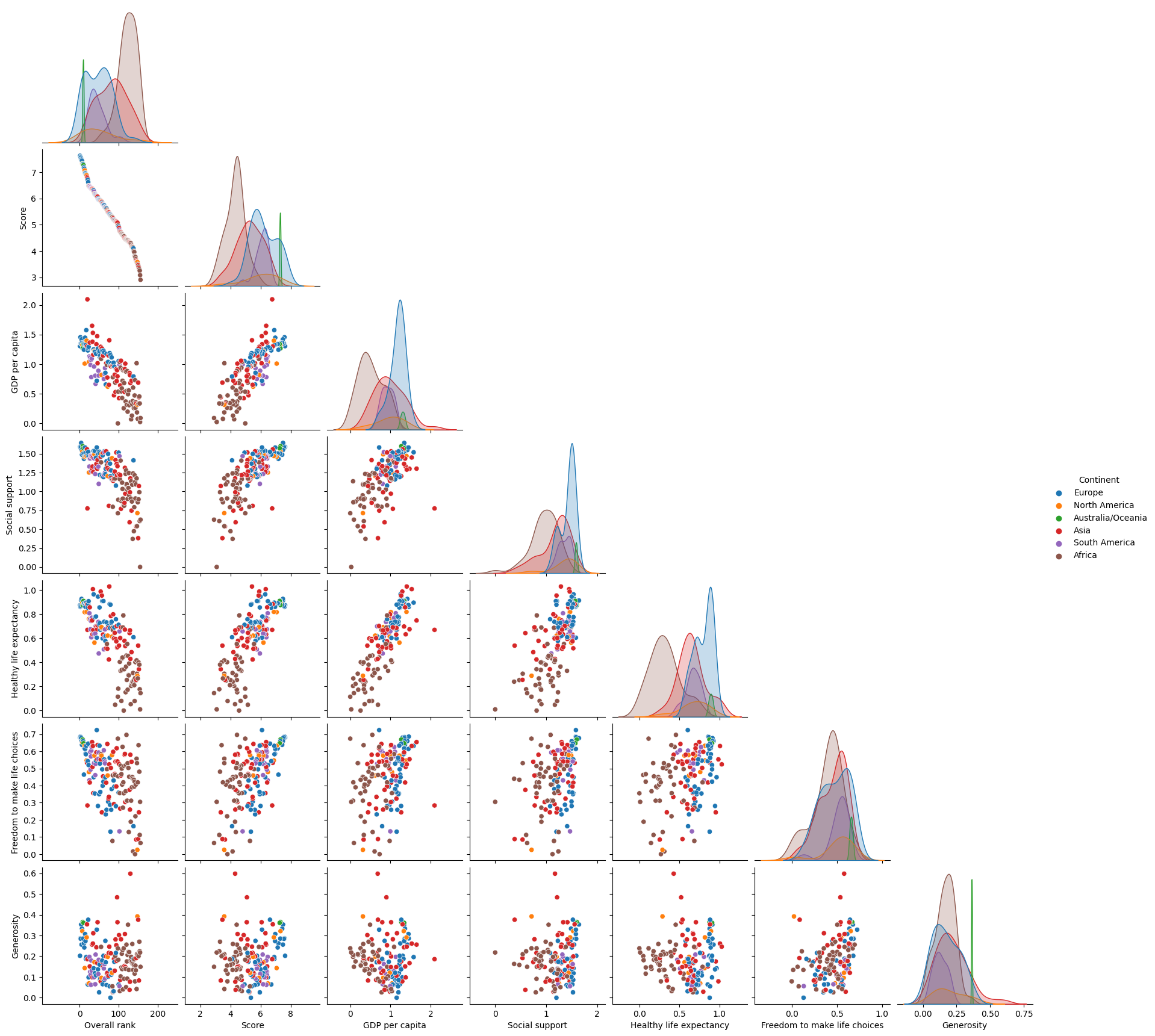
../../_images/74dc4872a74df100dd97148d4931558567bc38095c931df3141d6ab4f0bbd98e.png

I originally made the pairplot using all of the data columns in df, including those which we had added when creating predictions. This made the pairplot massive, with a lot of cross sections. Upon realizing this, I created a new Dataframe with only the original numeric data type columns. This allowed for a much better and far less chaotic visualization of the data in the pairplot.

As for what I am looking to gain out of analyzing this data, this happens to be the perfect kind of visualization. Though I could very well create several Altair charts for each combination of variables and find the line of best fit for each of them, this visualization allows me to easily see between two variables if there is a positive or negative relationship, or perhaps no discernible relationship at all. I am able to see a positive relationship between GDP per capita and Social support, and a negative relationship between Freedom to make life choices and Overall rank, just to name a few. These relationships make sense, and we can conclude with some confidence that there is a correlation between certain categories of data.

Summary#

As we can see, there are several factors with a relationship between them in the Happiness Index dataset. Some of these are subjective measures, however, and could be hard to fairly and accurately measure, such as “Generosity” and “Perceptions of corruption”. Much more, if they did vary from what they actually are (i.e. different data collection style, different measures for that category), it could greatly impact the country’s numerical ranking. Even GDP per capita can be hard to accurately measure, even though it is one of the most objective measures of the factors.

Through this project, I was able to conduct research on a topic and apply my knowledge from this class to another subject. As a Math major, I am not often exposed to other subjects, but I liked the interdisciplinary approach I could take with this, applying the methods of machine learning and data science to politics, economics, and society. I am appreciative of everything I’ve learned in this class, and have new insight to how useful data analysis can be.

References#

Your code above should include references. Here is some additional space for references.

Happiness Index 2018-2019, Sougata Pramanick, Kaggle https://www.kaggle.com/datasets/sougatapramanick/happiness-index-2018-2019?resource=download&select=2018.csv

World Heart Photo: https://www.google.com/url?sa=i&url=https://greatergood.berkeley.edu/article/item/world_happiness_report_finds_that_crises_make_us_kinder&psig=AOvVaw14PrJSHxr3An_VBfBHX_4e&ust=1686882826729000&source=images&cd=vfe&ved=0CAQQjB1qFwoTCNj397GexP8CFQAAAAAdAAAAABAD

User shajid01’s “Data Visualization using Seaborn” on the same dataset on Kaggle: https://www.kaggle.com/code/shajid01/data-visualization-using-seaborn

Seaborn Pairplot tutorial: https://towardsdatascience.com/seaborn-pairplot-enhance-your-data-understanding-with-a-single-plot-bf2f44524b22

Submission#

Using the Share button at the top right, enable Comment privileges for anyone with a link to the project. Then submit that link on Canvas.

Created in Deepnote