Week 9 Wednesday

Announcements

• Midterm 2 is Friday. Get a notecard if you need one.

• Jinghao will go over the sample midterm (posted on the Week 9 page) in discussion on Thursday. Sample solutions will be posted after discussion section.

• Worksheet 17 is posted. It is meant to get you started on the course project.

• Worksheet 18 is also posted. I recommend finishing this worksheet before Midterm 2, as it is mostly review material. Worksheet 18 is the last worksheet for Math 10.

• I have office hours starting at 12pm in here before the midterm on Friday.

• The specific new functions we introduce today will not be on Midterm 2, but the concepts are relevant.

import pandas as pd
import altair as alt

Temperature data set

Here is the dataset we finished with on Friday. We have succeeded in plotting the data, but we haven’t done any Machine Learning with the data yet.

We would really like to use a line like color="city", so that temperatures in different cities get different colors. We can’t do that with the current version of the DataFrame, because the city names are given in column names (as opposed to being given in their own column).

df_pre = pd.read_csv("temperature_f.csv", parse_dates=["datetime"])
df_pre.sample(4, random_state=0)

	datetime	Vancouver	Portland	San Francisco	Seattle	Los Angeles	San Diego	Las Vegas	Phoenix	Albuquerque	...	Philadelphia	New York	Montreal	Boston	Beersheba	Tel Aviv District	Eilat	Haifa	Nahariyya	Jerusalem
37037	2016-12-22 18:00:00	38.7	31.7	52.9	34.9	55.3	60.9	45.6	60.8	34.1	...	46.8	43.6	32.0	36.4	44.3	58.4	57.5	55.4	55.4	58.7
23197	2015-05-26 02:00:00	61.6	60.6	56.2	60.3	65.7	64.0	75.3	78.4	60.3	...	75.0	73.2	62.5	66.9	58.2	59.7	71.4	69.9	69.9	65.1
33027	2016-07-08 16:00:00	59.9	62.0	59.3	59.9	70.9	70.5	90.6	95.2	79.6	...	87.7	83.8	69.4	66.5	87.3	87.4	104.4	97.0	79.0	87.4
22542	2015-04-28 19:00:00	50.6	55.1	57.0	56.8	79.2	82.3	74.1	78.5	51.3	...	63.6	63.6	58.7	50.8	75.0	70.7	74.1	70.7	66.9	70.6

4 rows × 37 columns

Originally the city names appear as column headers. For both Altair and scikit-learn, we want a column containing all these city names.

df_melted = df_pre.melt(
        id_vars="datetime",
        var_name="city", 
        value_name="temperature"
    )

By using the method melt, we have gotten a much longer version of the DataFrame, that now has just three columns. The “city” column contains the old column headers (repeated many times each city), and the “temperature” column contains the old cell contents.

df_melted.sample(4, random_state=0)

	datetime	city	temperature
1478577	2016-03-25 22:00:00	Eilat	78.0
1299334	2016-06-07 11:00:00	Montreal	61.1
1072194	2016-05-01 19:00:00	Miami	84.5
863753	2013-03-15 18:00:00	Atlanta	48.5

The resulting DataFrame is much longer.

Here we check using an f-string. We use triple quotation marks so that we are allowed to include a line break in the string.

print(f"""The original DataFrame had shape {df_pre.shape}. 
The new DataFrame has shape {df_melted.shape}.""")

The original DataFrame had shape (45252, 37). 
The new DataFrame has shape (1629072, 3).

Here is what we did on Friday, although I’m naming the final DataFrame df3 instead of df, because I want to make more changes before calling the result df.

• Keep only the rows corresponding to the cities in the following cities list.

• Drop the rows with missing values.

• Sort the DataFrame by date.

• Name the resulting DataFrame df3.

cities = ["San Diego", "San Francisco", "Detroit"]

We keep only the rows corresponding to those three cities using Boolean indexing and the isin method. We then drop the rows with missing values. We then sort the values by date. (Probably the sorting would not be correct if the dates were strings instead of datetime objects.)

df1 = df_melted[df_melted["city"].isin(cities)]
df2 = df1.dropna(axis=0)
df3 = df2.sort_values("datetime")

Here is how the resulting DataFrame df3 looks. Notice how the first three rows are all from the same row and at 1pm. Then in the last row it moves to 2pm. (It does seem like the DataFrame is sorted by date, and we are only seeing the three listed cities, unlike earlier when we saw many different cities.)

df3.head(4)

	datetime	city	temperature
90504	2012-10-01 13:00:00	San Francisco	61.4
226260	2012-10-01 13:00:00	San Diego	65.1
905040	2012-10-01 13:00:00	Detroit	51.6
905041	2012-10-01 14:00:00	Detroit	51.7

Plotting the data

Now that we have “melted” the DataFrame, it is easy to plot using Altair.

Our goal is to predict these values using scikit-learn. This will be our first time using a decision tree for regression (as opposed to classification).

c_true = alt.Chart(df3[6400:7000]).mark_line().encode(
    x="datetime",
    y="temperature",
    color="city",
    tooltip=["city", "temperature", "datetime"]
).properties(
    width=600
)

c_true

Adding Boolean columns for the cities

Because the “city” column contains strings, we can’t use it as an input when fitting a decision tree. We will convert it to multiple Boolean indicator columns.

Here are two options:

• Use pd.get_dummies.

• Use scikit-learn’s OneHotEncoder class.

I couldn’t immediately get OneHotEncoder to work with Pipeline (according to ChatGPT, it seems to require yet another tool called ColumnTransformer), so I’m going to use the pandas option.

• Make a new DataFrame df4 containing Boolean indicator columns for the “city” values using the pandas function get_dummies.

I couldn’t remember the name of the keyword argument I wanted to use, so I called the following help function. This reminded me that columns was the keyword argument I wanted to use.

help(pd.get_dummies)

Help on function get_dummies in module pandas.core.reshape.reshape:

get_dummies(data, prefix=None, prefix_sep='_', dummy_na=False, columns=None, sparse=False, drop_first=False, dtype=None) -> 'DataFrame'
    Convert categorical variable into dummy/indicator variables.
    
    Parameters
    ----------
    data : array-like, Series, or DataFrame
        Data of which to get dummy indicators.
    prefix : str, list of str, or dict of str, default None
        String to append DataFrame column names.
        Pass a list with length equal to the number of columns
        when calling get_dummies on a DataFrame. Alternatively, `prefix`
        can be a dictionary mapping column names to prefixes.
    prefix_sep : str, default '_'
        If appending prefix, separator/delimiter to use. Or pass a
        list or dictionary as with `prefix`.
    dummy_na : bool, default False
        Add a column to indicate NaNs, if False NaNs are ignored.
    columns : list-like, default None
        Column names in the DataFrame to be encoded.
        If `columns` is None then all the columns with
        `object` or `category` dtype will be converted.
    sparse : bool, default False
        Whether the dummy-encoded columns should be backed by
        a :class:`SparseArray` (True) or a regular NumPy array (False).
    drop_first : bool, default False
        Whether to get k-1 dummies out of k categorical levels by removing the
        first level.
    dtype : dtype, default np.uint8
        Data type for new columns. Only a single dtype is allowed.
    
    Returns
    -------
    DataFrame
        Dummy-coded data.
    
    See Also
    --------
    Series.str.get_dummies : Convert Series to dummy codes.
    
    Examples
    --------
    >>> s = pd.Series(list('abca'))
    
    >>> pd.get_dummies(s)
       a  b  c
    0  1  0  0
    1  0  1  0
    2  0  0  1
    3  1  0  0
    
    >>> s1 = ['a', 'b', np.nan]
    
    >>> pd.get_dummies(s1)
       a  b
    0  1  0
    1  0  1
    2  0  0
    
    >>> pd.get_dummies(s1, dummy_na=True)
       a  b  NaN
    0  1  0    0
    1  0  1    0
    2  0  0    1
    
    >>> df = pd.DataFrame({'A': ['a', 'b', 'a'], 'B': ['b', 'a', 'c'],
    ...                    'C': [1, 2, 3]})
    
    >>> pd.get_dummies(df, prefix=['col1', 'col2'])
       C  col1_a  col1_b  col2_a  col2_b  col2_c
    0  1       1       0       0       1       0
    1  2       0       1       1       0       0
    2  3       1       0       0       0       1
    
    >>> pd.get_dummies(pd.Series(list('abcaa')))
       a  b  c
    0  1  0  0
    1  0  1  0
    2  0  0  1
    3  1  0  0
    4  1  0  0
    
    >>> pd.get_dummies(pd.Series(list('abcaa')), drop_first=True)
       b  c
    0  0  0
    1  1  0
    2  0  1
    3  0  0
    4  0  0
    
    >>> pd.get_dummies(pd.Series(list('abc')), dtype=float)
         a    b    c
    0  1.0  0.0  0.0
    1  0.0  1.0  0.0
    2  0.0  0.0  1.0

Here is a reminder of how the top of the data looks.

df3.head(4)

	datetime	city	temperature
90504	2012-10-01 13:00:00	San Francisco	61.4
226260	2012-10-01 13:00:00	San Diego	65.1
905040	2012-10-01 13:00:00	Detroit	51.6
905041	2012-10-01 14:00:00	Detroit	51.7

Here is the result of calling the get_dummies function for the “city” column. This is a common procedure in Machine Learning. We have a column with data we want to use as an input (in this case, we want to use the city), but we aren’t able to because the data is not numeric. Here we add a column for each city, indicating if the row corresponded to that particular city. For example, notice that our DataFrame begins “not Detroit”, “not Detroit”, “Detroit”, “Detroit”. This corresponds to the “city_Detroit” column beginning [0, 0, 1, 1]. I think of this as being equivalent to [False, False, True, True].

The main point is that we can use these three new columns as inputs to our Machine Learning algorithm.

pd.get_dummies(df3, columns=["city"])

	datetime	temperature	city_Detroit	city_San Diego	city_San Francisco
90504	2012-10-01 13:00:00	61.4	0	0	1
226260	2012-10-01 13:00:00	65.1	0	1	0
905040	2012-10-01 13:00:00	51.6	1	0	0
905041	2012-10-01 14:00:00	51.7	1	0	0
90505	2012-10-01 14:00:00	61.4	0	0	1
...	...	...	...	...	...
271509	2017-11-29 22:00:00	67.0	0	1	0
950290	2017-11-29 23:00:00	40.8	1	0	0
271510	2017-11-29 23:00:00	67.0	0	1	0
271511	2017-11-30 00:00:00	64.8	0	1	0
950291	2017-11-30 00:00:00	38.2	1	0	0

134964 rows × 5 columns

We are doing the same thing in the next cell, the only difference being that we save the result with the variable name df4.

df4 = pd.get_dummies(df3, columns=["city"])

• Make a list city_cols containing the three new column names we just added.

Here is how we can make that list using list comprehension.

city_cols = [c for c in df4.columns if c.startswith("city_")]
city_cols

['city_Detroit', 'city_San Diego', 'city_San Francisco']

The following alternative approach doesn’t seem as robust, because we need to know there are three columns, and we need to know they’re at the end of the DataFrame. On the other hand, with the following approach, we don’t need to know that the column names start with "city_".

df4.columns[-3:]

Index(['city_Detroit', 'city_San Diego', 'city_San Francisco'], dtype='object')

• Add the “city” column back in (so we can use it with plotting) using pd.concat with an appropriate axis keyword argument. Name the resulting DataFrame df_ext (for “extended”).

Unfortunately the following error is a little difficult to interpret. It is implying that df3[["city"]] is being treated like an axis argument.

pd.concat(df4, df3[["city"]], axis=1)

---------------------------------------------------------------------------
TypeError                                 Traceback (most recent call last)
/tmp/ipykernel_106/1418832173.py in <module>
----> 1 pd.concat(df4, df3[["city"]], axis=1)

TypeError: concat() got multiple values for argument 'axis'

The DataFrames we want to merge together are supposed to be grouped together, for example in a list or a tuple. Here we put them into a tuple.

Notice also that we use the keyword argument axis=1, because we are changing the column labels and keeping the row labels the same. (We are including a new column label, the label “city”.)

df_ext = pd.concat((df4, df3[["city"]]), axis=1)
df_ext

	datetime	temperature	city_Detroit	city_San Diego	city_San Francisco	city
90504	2012-10-01 13:00:00	61.4	0	0	1	San Francisco
226260	2012-10-01 13:00:00	65.1	0	1	0	San Diego
905040	2012-10-01 13:00:00	51.6	1	0	0	Detroit
905041	2012-10-01 14:00:00	51.7	1	0	0	Detroit
90505	2012-10-01 14:00:00	61.4	0	0	1	San Francisco
...	...	...	...	...	...	...
271509	2017-11-29 22:00:00	67.0	0	1	0	San Diego
950290	2017-11-29 23:00:00	40.8	1	0	0	Detroit
271510	2017-11-29 23:00:00	67.0	0	1	0	San Diego
271511	2017-11-30 00:00:00	64.8	0	1	0	San Diego
950291	2017-11-30 00:00:00	38.2	1	0	0	Detroit

134964 rows × 6 columns

Adding numeric columns related to “datetime”

We also want to be able to use the month, the hour, etc, as inputs to our decision tree. We add these as new columns to a DataFrame. Notice that we are are using numbers (from day_of_week), like 0, rather than strings (from day_name()) like "Monday".

• Define df to be a copy of df_ext.

(Why are we using all these different names, like df1, df2, df_ext, …? This way if we make a mistake at one step, we don’t destroy the preceding DataFrame. If I were preparing a finalized version of this notebook, I would probably call all of them df. If we were to use df = df_ext instead of df = df_ext.copy(), that would not work, because for example adding a column to df would add a column to df_ext at the same time.)

df = df_ext.copy()

• For each of the following df["datetime"].dt attributes, add a corresponding column to df. Notice that the results are numeric.

var_cols = ["year", "day", "month", "hour", "day_of_week"]

Here is an example of what we want to do, but how can we do this with less repetition.

df["day"] = df["datetime"].dt.day
df["month"] = df["datetime"].dt.month

Notice for example how these dates at the top of the DataFrame df are in October, and our new “month” column starts with 10.

df.head(4)

	datetime	temperature	city_Detroit	city_San Diego	city_San Francisco	city	day	month
90504	2012-10-01 13:00:00	61.4	0	0	1	San Francisco	1	10
226260	2012-10-01 13:00:00	65.1	0	1	0	San Diego	1	10
905040	2012-10-01 13:00:00	51.6	1	0	0	Detroit	1	10
905041	2012-10-01 14:00:00	51.7	1	0	0	Detroit	1	10

Here are the five columns we want to add.

var_cols = ["year", "day", "month", "hour", "day_of_week"]

The first attempt does not work, because even if var = "year" for example, evaluating df["datetime"].dt.var will not have anything to do with “year”, it will be looking for an attribute named var.

for var in var_cols:
    df[var] = df["datetime"].dt.var

---------------------------------------------------------------------------
AttributeError                            Traceback (most recent call last)
/tmp/ipykernel_106/497635513.py in <module>
      1 for var in var_cols:
----> 2     df[var] = df["datetime"].dt.var

AttributeError: 'DatetimeProperties' object has no attribute 'var'

I then tried using square brackets, but that also does not work.

for var in var_cols:
    df[var] = df["datetime"].dt[var]

---------------------------------------------------------------------------
TypeError                                 Traceback (most recent call last)
/tmp/ipykernel_106/1090741701.py in <module>
      1 for var in var_cols:
----> 2     df[var] = df["datetime"].dt[var]

TypeError: 'DatetimeProperties' object is not subscriptable

Here is a solution that works. We use the built-in function getattr. (This isn’t a Machine Learning or Data Science topic, this is a Python topic.)

for var in var_cols:
    df[var] = getattr(df["datetime"].dt, var)

Here we can see the 5 new columns we added. We will use these columns and our city indicator columns as our predictors for our decision tree.

df.head(4)

	datetime	temperature	city_Detroit	city_San Diego	city_San Francisco	city	day	month	year	hour	day_of_week
90504	2012-10-01 13:00:00	61.4	0	0	1	San Francisco	1	10	2012	13	0
226260	2012-10-01 13:00:00	65.1	0	1	0	San Diego	1	10	2012	13	0
905040	2012-10-01 13:00:00	51.6	1	0	0	Detroit	1	10	2012	13	0
905041	2012-10-01 14:00:00	51.7	1	0	0	Detroit	1	10	2012	14	0

Predicting temperature using DecisionTreeRegressor

We want to use the “datetime” column and the “city” column. We need to convert the “city” column to (multiple) Boolean columns before we can use it as an input.

• Make a list cols containing the columns in city_cols and in var_cols.

It’s easy to concatenate two lists: just use +. This new list cols will be our input features.

cols = city_cols + var_cols
cols

['city_Detroit',
 'city_San Diego',
 'city_San Francisco',
 'year',
 'day',
 'month',
 'hour',
 'day_of_week']

• Fit a DecisionTreeRegressor object with a maximum of 16 leaf nodes to the data in these columns (notice that they’re all numeric). Use “temperature” as our target.

This is our first time using a DecisionTreeRegressor, but it works very similarly to DecisionTreeClassifier. The main difference is that the target values in the regression case should be numbers.

from sklearn.tree import DecisionTreeRegressor

Here we instantiate the regressor, specifying the maximum number of leaf nodes.

reg = DecisionTreeRegressor(max_leaf_nodes=16)

Here we fit the regressor, using “temperature” as our target.

reg.fit(df[cols], df["temperature"])

DecisionTreeRegressor(max_leaf_nodes=16)

• Add a “pred” column to df containing the predicted temperatures.

df["pred"] = reg.predict(df[cols])

• Plot the data using the following.

alt.Chart(df[6400:7000]).mark_line().encode(
    x="datetime",
    y="pred",
    color="city",
    tooltip=["city", "temperature", "pred", "datetime", "hour"]
).properties(
    width=600
)

This is just one small portion of the data, corresponding to about one week. Notice how we only see San Francisco and Detroit. That is because the predictions for San Francisco and San Diego are the same.

Also, because we used a maximum of 16 leaf nodes, there are a maximum of 16 values that can be predicted. That is why we see so many flat line segments in this chart.

alt.Chart(df[6400:7000]).mark_line().encode(
    x="datetime",
    y="pred",
    color="city",
    tooltip=["city", "temperature", "pred", "datetime", "hour"]
).properties(
    width=600
)

• Can you see where the predicted values come from, using the following diagram?

(We will need to change clf to something else.)

import matplotlib.pyplot as plt
from sklearn.tree import plot_tree

fig = plt.figure(figsize=(20,10))
_ = plot_tree(clf, 
                   feature_names=clf.feature_names_in_,
                   filled=False)

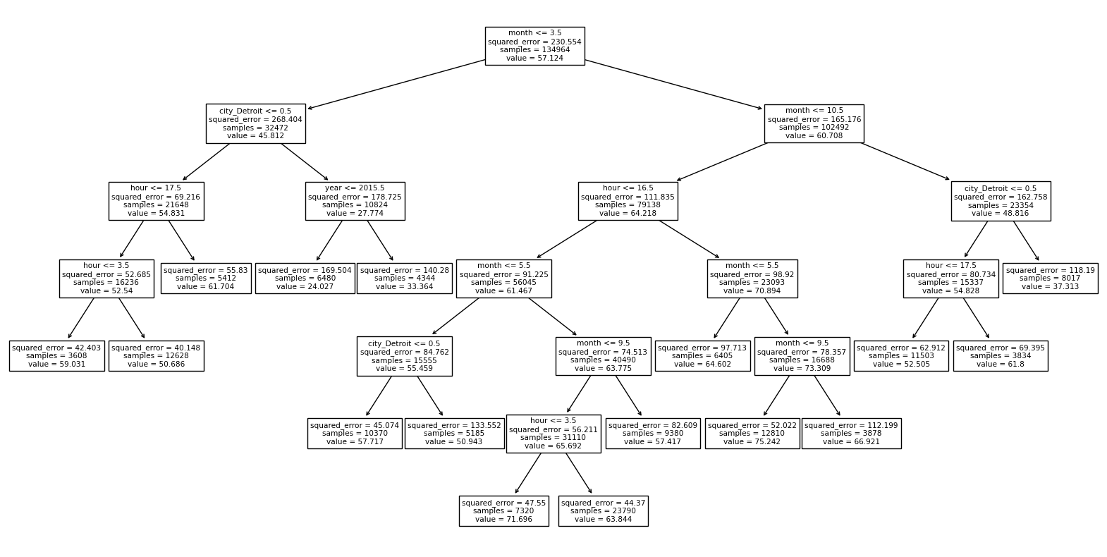
Using the Altair tooltip, I focused on a point for San Francisco on January 1st at 7am. Following the diagram, we wind up near the lower-left portion of the diagram, with value 50.686. This is indeed the predicted temperature for the point we were looking at. For the particular point I was looking at, the true temperature was 42.3.

import matplotlib.pyplot as plt
from sklearn.tree import plot_tree

fig = plt.figure(figsize=(20,10))
_ = plot_tree(reg, 
                   feature_names=reg.feature_names_in_,
                   filled=False)

• How does the Altair chart change if you use a max depth of 14 instead of a max leaf nodes of 16? (Don’t try to make the tree diagram in this case.)

This might sound similar, but it is extremely different.

reg = DecisionTreeRegressor(max_depth=14)

reg.fit(df[cols], df["temperature"])

DecisionTreeRegressor(max_depth=14)

df["pred"] = reg.predict(df[cols])

Here is the chart. Recall how above the same predictions were made for San Diego and San Francisco (at least in the part of the chart we are plotting). Here there are many different values plotted.

c_14 = alt.Chart(df[6400:7000]).mark_line().encode(
    x="datetime",
    y="pred",
    color="city",
    tooltip=["city", "temperature", "pred", "datetime", "hour"]
).properties(
    width=600
)

c_14

How do those values compare to the true values? Look how similar they are! Is that a good sign? No, it is almost surely a sign of overfitting. Using a depth of 14 in this case is providing too much flexibility to the model.

c_true + c_14

• How many leaf nodes are there in this case? Use the method get_n_leaves.

reg.get_n_leaves()

12722

The theoretical maximum number of leaf nodes for a depth of 14 is \(2^{14}\).

2**14

16384

• Do you think this new decision tree would do well at predicting unseen data?

No, I would expect poor performance on new data, because it is overfitting the input data.

• I don’t think using train_test_split makes much sense on this data, do you see why?

Imagine we separate the data into a training set and a test set. Maybe the training set includes the data from 7am (for a particular city and day) and the test set includes the data from 8am (for that same city and day). In real life, the temperatures for 7am and 8am will be very similar, so we will probably get a very accurate prediction for the 8am value, but I do not think that is meaningful. (Another way to think about it, is if we want to predict the temperature at some day in the future, we will not know what the temperature is one hour earlier.)

In short, if 7am is in the training set, it’s like we already knew the 8am value.

I believe a better way with this sort of data (this is called time series data): remove a whole month or a whole year, and see how we do on the predictions for that missing month or year. That performance would be much more indicative of how we might hope to do on new predictions in the future.

We didn’t get to the following.

Extra time?

I doubt we will get here, but if we do, this will give a sense of how decision trees make their predictions. (Not how they make their cuts.)

• Make a new decision tree regressor that allows only 4 leaf nodes.

• Draw the corresponding diagram using plot_tree.

• Can you recover the given value for one of the leaf nodes using Boolean indexing?