Predict the Month through London Weather¶

Author: Jie Lin

Course Project, UC Irvine, Math 10, S22

Introduction¶

In this project, I tried to use the dataset “london_weather” to explore how can we predict the specific month of london through serveral weather factors. Besides, I also explored the importance of each factor in predicting months. In addition, I explored the most common mistakes in predicting months.

Main portion of the project¶

(You can either have all one section or divide into multiple sections)

Here, I import the necessary library for this project.

import altair as alt
import pandas as pd
import matplotlib.pyplot as plt
from pandas.api.types import is_numeric_dtype
from sklearn.linear_model import LogisticRegression
from sklearn.model_selection import train_test_split
from sklearn.tree import DecisionTreeClassifier
from sklearn.tree import plot_tree
from sklearn.neighbors import KNeighborsClassifier
from sklearn.metrics import log_loss
from sklearn.preprocessing import StandardScaler

First, I need to download the dataset and deal with same data in this dataset.

df = pd.read_csv('london_weather.csv')

Here, I remove all the missing values in this dataset.

df=df.dropna() 

df

	date	cloud_cover	sunshine	global_radiation	max_temp	mean_temp	min_temp	precipitation	pressure	snow_depth
0	19790101	2.0	7.0	52.0	2.3	-4.1	-7.5	0.4	101900.0	9.0
1	19790102	6.0	1.7	27.0	1.6	-2.6	-7.5	0.0	102530.0	8.0
2	19790103	5.0	0.0	13.0	1.3	-2.8	-7.2	0.0	102050.0	4.0
3	19790104	8.0	0.0	13.0	-0.3	-2.6	-6.5	0.0	100840.0	2.0
4	19790105	6.0	2.0	29.0	5.6	-0.8	-1.4	0.0	102250.0	1.0
...	...	...	...	...	...	...	...	...	...	...
14970	20191227	8.0	0.0	12.0	9.6	7.5	6.6	0.0	102880.0	0.0
14971	20191228	8.0	0.0	12.0	9.9	8.1	6.6	0.0	103630.0	0.0
14972	20191229	6.0	2.2	29.0	11.5	8.7	7.4	0.0	103360.0	0.0
14973	20191230	0.0	3.6	37.0	9.3	6.5	1.5	0.0	102970.0	0.0
14974	20191231	7.0	0.0	13.0	9.4	7.1	4.9	0.0	103160.0	0.0

13843 rows × 10 columns

df.columns

Index(['date', 'cloud_cover', 'sunshine', 'global_radiation', 'max_temp',
       'mean_temp', 'min_temp', 'precipitation', 'pressure', 'snow_depth'],
      dtype='object')

Then I covert number in the column named “date” to a pandas datetime object.

df["date"]=pd.to_datetime(df["date"], format='%Y%m%d')

I plan to find out all the columns with numbers and arrange the name of these columns as a set.

num_cols = [c for c in df.columns if is_numeric_dtype(df[c])]

num_cols

['cloud_cover',
 'sunshine',
 'global_radiation',
 'max_temp',
 'mean_temp',
 'min_temp',
 'precipitation',
 'pressure',
 'snow_depth']

Then I plan to add a new column named “Month”, which contains the correspondintg month to the datetime in the “date” column.

df["Month"]=df["date"].dt.month

df

	date	cloud_cover	sunshine	global_radiation	max_temp	mean_temp	min_temp	precipitation	pressure	snow_depth	Month
0	1979-01-01	2.0	7.0	52.0	2.3	-4.1	-7.5	0.4	101900.0	9.0	1
1	1979-01-02	6.0	1.7	27.0	1.6	-2.6	-7.5	0.0	102530.0	8.0	1
2	1979-01-03	5.0	0.0	13.0	1.3	-2.8	-7.2	0.0	102050.0	4.0	1
3	1979-01-04	8.0	0.0	13.0	-0.3	-2.6	-6.5	0.0	100840.0	2.0	1
4	1979-01-05	6.0	2.0	29.0	5.6	-0.8	-1.4	0.0	102250.0	1.0	1
...	...	...	...	...	...	...	...	...	...	...	...
14970	2019-12-27	8.0	0.0	12.0	9.6	7.5	6.6	0.0	102880.0	0.0	12
14971	2019-12-28	8.0	0.0	12.0	9.9	8.1	6.6	0.0	103630.0	0.0	12
14972	2019-12-29	6.0	2.2	29.0	11.5	8.7	7.4	0.0	103360.0	0.0	12
14973	2019-12-30	0.0	3.6	37.0	9.3	6.5	1.5	0.0	102970.0	0.0	12
14974	2019-12-31	7.0	0.0	13.0	9.4	7.1	4.9	0.0	103160.0	0.0	12

13843 rows × 11 columns

Here I create a copy of df and I plan to use this copy in the following steps.

df1=df.copy()
df2=df.copy()
df3=df.copy()

Using Logistic Regression to Predict¶

Then, I plan to use all columns that contains numbers related to the weather of different days to predict the possible month of each day by using LogisticRegression.

reg=LogisticRegression()

reg.fit(df[num_cols],df["Month"])

/shared-libs/python3.7/py/lib/python3.7/site-packages/sklearn/linear_model/_logistic.py:818: ConvergenceWarning: lbfgs failed to converge (status=1):
STOP: TOTAL NO. of ITERATIONS REACHED LIMIT.

Increase the number of iterations (max_iter) or scale the data as shown in:
    https://scikit-learn.org/stable/modules/preprocessing.html
Please also refer to the documentation for alternative solver options:
    https://scikit-learn.org/stable/modules/linear_model.html#logistic-regression
  extra_warning_msg=_LOGISTIC_SOLVER_CONVERGENCE_MSG,

LogisticRegression()

Then I create a new column named “Pred” which contains the values that Logistic Regression predict the corresponding months to days by the data from the columns that contains data related to the weather of a day.

df1["Pred"]=reg.predict(df[num_cols])

df1

	date	cloud_cover	sunshine	global_radiation	max_temp	mean_temp	min_temp	precipitation	pressure	snow_depth	Month	Pred
0	1979-01-01	2.0	7.0	52.0	2.3	-4.1	-7.5	0.4	101900.0	9.0	1	2
1	1979-01-02	6.0	1.7	27.0	1.6	-2.6	-7.5	0.0	102530.0	8.0	1	1
2	1979-01-03	5.0	0.0	13.0	1.3	-2.8	-7.2	0.0	102050.0	4.0	1	12
3	1979-01-04	8.0	0.0	13.0	-0.3	-2.6	-6.5	0.0	100840.0	2.0	1	12
4	1979-01-05	6.0	2.0	29.0	5.6	-0.8	-1.4	0.0	102250.0	1.0	1	1
...	...	...	...	...	...	...	...	...	...	...	...	...
14970	2019-12-27	8.0	0.0	12.0	9.6	7.5	6.6	0.0	102880.0	0.0	12	12
14971	2019-12-28	8.0	0.0	12.0	9.9	8.1	6.6	0.0	103630.0	0.0	12	12
14972	2019-12-29	6.0	2.2	29.0	11.5	8.7	7.4	0.0	103360.0	0.0	12	1
14973	2019-12-30	0.0	3.6	37.0	9.3	6.5	1.5	0.0	102970.0	0.0	12	11
14974	2019-12-31	7.0	0.0	13.0	9.4	7.1	4.9	0.0	103160.0	0.0	12	12

13843 rows × 12 columns

Here I compare the data of true month of days to the data of predict months of days.

pd.Series(df1['Pred']==df1['Month']).astype(float).mean()

0.2786968142743625

From the result of the comparision of the data of true months of days to the data of predict months of days, we could see that there are only 27.8698% rows matches to each other, which is a low percetage, which reveals that Logistic Regression may not be a good way to predict the month.

Using Decision Tree Classifier to Predict¶

since we found out that LogisticRegression does not work well for predicting the corresponding months, I plan to try to use DecisionTreeClassifier to predict the corresponding month.

First, I make a new copy of df and build the train and test sets.

df2=df.copy()

X_train, X_test, y_train, y_test = train_test_split(
    df2[num_cols],
    df2["Month"],
    test_size=0.2,
    random_state=0
)

for nodes in range(100,5000,50):
    clf = DecisionTreeClassifier(max_depth=10, max_leaf_nodes=nodes)
    clf.fit(X_train, y_train)
    a = clf.score(X_train, y_train)
    b = clf.score(X_test, y_test)
    print (a,b)# not overfitting

6396965865992414 0.5868544600938967
6854795015351274 0.625496569158541
7125699837457107 0.647887323943662
7327975437962796 0.656554712892741
7467942929384143 0.659443842542434
7564565649268556 0.6601661249548574
7650352176268738 0.6576381365113759
7716272349647824 0.6569158540989527
7769550297995305 0.6587215601300108
7812895069532237 0.6598049837486457
7832761423153333 0.6587215601300108
7834567455300704 0.6561935716865295
7833664439227018 0.6569158540989527
7832761423153333 0.659443842542434
7835470471374391 0.6587215601300108
7834567455300704 0.6590827013362225
7832761423153333 0.6576381365113759
7832761423153333 0.6572769953051644
7834567455300704 0.6583604189237992
7834567455300704 0.6587215601300108
7834567455300704 0.6583604189237992
7832761423153333 0.6590827013362225
7831858407079646 0.659443842542434
7833664439227018 0.659443842542434
7834567455300704 0.6572769953051644
7836373487448076 0.6583604189237992
7833664439227018 0.6579992777175876
7836373487448076 0.6569158540989527
7832761423153333 0.659443842542434
7831858407079646 0.6572769953051644
7833664439227018 0.6590827013362225
7832761423153333 0.6590827013362225
7835470471374391 0.6598049837486457
7832761423153333 0.6583604189237992
7832761423153333 0.6576381365113759
7834567455300704 0.656554712892741
7835470471374391 0.6572769953051644
7834567455300704 0.6587215601300108
7831858407079646 0.6587215601300108
7833664439227018 0.6569158540989527
7835470471374391 0.6572769953051644
7832761423153333 0.6583604189237992
7832761423153333 0.6587215601300108
7834567455300704 0.6572769953051644
7836373487448076 0.6583604189237992
7834567455300704 0.6576381365113759
7834567455300704 0.6572769953051644
7833664439227018 0.6558324304803178
7833664439227018 0.6583604189237992
7833664439227018 0.659443842542434
7834567455300704 0.6587215601300108
7834567455300704 0.659443842542434
7832761423153333 0.6583604189237992
7833664439227018 0.659443842542434
7832761423153333 0.6587215601300108
7833664439227018 0.6576381365113759
7833664439227018 0.6576381365113759
7833664439227018 0.6572769953051644
7833664439227018 0.6576381365113759
7832761423153333 0.6576381365113759
7834567455300704 0.659443842542434
7833664439227018 0.6569158540989527
7831858407079646 0.6561935716865295
7833664439227018 0.6576381365113759
7834567455300704 0.6569158540989527
7834567455300704 0.6583604189237992
7832761423153333 0.6583604189237992
7836373487448076 0.6576381365113759
7836373487448076 0.6587215601300108
7835470471374391 0.6590827013362225
7836373487448076 0.6561935716865295
7833664439227018 0.656554712892741
7832761423153333 0.6587215601300108
7835470471374391 0.6583604189237992
7832761423153333 0.6579992777175876
7831858407079646 0.6558324304803178
7833664439227018 0.6579992777175876
7835470471374391 0.6583604189237992
7833664439227018 0.6601661249548574
7834567455300704 0.6558324304803178
7835470471374391 0.6572769953051644
7833664439227018 0.6583604189237992
7834567455300704 0.6569158540989527
7833664439227018 0.6579992777175876
7833664439227018 0.656554712892741
7836373487448076 0.6572769953051644
7832761423153333 0.6576381365113759
7832761423153333 0.6558324304803178
7834567455300704 0.6587215601300108
7834567455300704 0.6572769953051644
7834567455300704 0.656554712892741
7833664439227018 0.659443842542434
7834567455300704 0.6587215601300108
7832761423153333 0.6587215601300108
7834567455300704 0.6590827013362225
7833664439227018 0.6572769953051644
7832761423153333 0.6569158540989527
7834567455300704 0.6583604189237992

From the result of above code, we could see that when max_leaf_nodes in the range (100,5000) with interval 50, the possibility that train data predict correctly is always around 0.78 while the possibility that the test data predict correctly is always around 0.65 to 0.66. therefore, there does not exist overfiting.

Since there is no overfiting, i randomly picks one value from range (100,500) with interval 50 and I want to use this setting to draw a picture of the decision tree.

clf = DecisionTreeClassifier(max_depth=10, max_leaf_nodes=600)

clf.fit(X_train, y_train)

DecisionTreeClassifier(max_depth=10, max_leaf_nodes=600)

clf.score(X_train, y_train)

0.7831858407079646

clf.score(X_test, y_test)

0.6579992777175876

from sklearn.tree import plot_tree

import matplotlib.pyplot as plt

fig = plt.figure(figsize=(10,20))
plot_tree(
    clf,
    feature_names=clf.feature_names_in_,
    filled=True
);

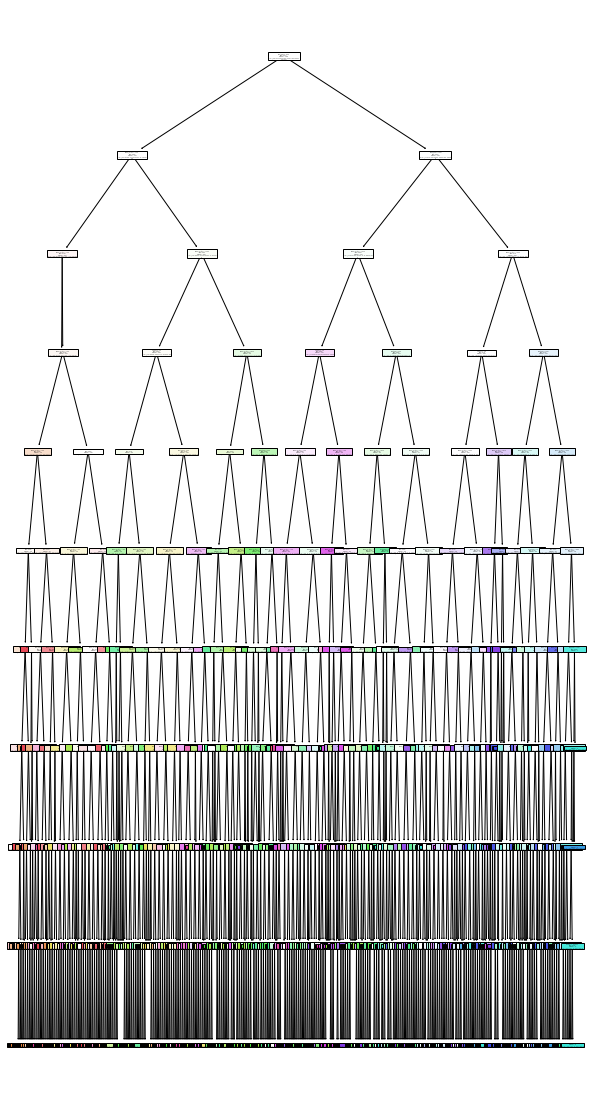
Figure out Importance of Each Factor¶

Then, I am a little curious about the importance of each weather factor in predicting the month. Therefore, plan to figure out the importance of each weather factor in predicting the weather.

pd.Series(clf.feature_importances_, index=num_cols)

cloud_cover         0.008456
sunshine            0.321073
global_radiation    0.410099
max_temp            0.133289
mean_temp           0.074589
min_temp            0.031777
precipitation       0.006093
pressure            0.014625
snow_depth          0.000000
dtype: float64

df_feat = pd.DataFrame({"importance": clf.feature_importances_, "feature": clf.feature_names_in_})

alt.Chart(df_feat).mark_bar().encode(
    x="importance",
    y="feature"
).properties(
    title = 'Feature Importance'
)

From the code of the above result, we could see that the most two importance weather factors in prediciting months is global_radiation and sunshine.

f1 = []
for i in y_test.index:
    f1.append(df['sunshine'][i])

f2 = []
for i in y_test.index:
    f2.append(df['global_radiation'][i])

f3 = []
for i in y_test.index:
    f3.append(df['date'][i])

df_true = pd.DataFrame()
df_true['sunshine'] = f1
df_true['global_radiation'] = f2
df_true['date']=f3
df_true['Month'] = list(y_test)

df_pred = pd.DataFrame()
df_pred['sunshine'] = f1
df_pred['global_radiation'] = f2
df_pred['date']=f3
df_pred['Predict'] = clf.predict(X_test)

alt.data_transformers.enable('default', max_rows=None)

DataTransformerRegistry.enable('default')

sel = alt.selection_single(fields=["Month"])
sel1 = alt.selection_single(fields=["Predict"])

c1=alt.Chart(df_true).mark_circle().encode(
    x=alt.X("sunshine", scale=alt.Scale(zero=False)),
    y=alt.Y("global_radiation", scale=alt.Scale(zero=False)),
    color=alt.Color("Month:O",scale=alt.Scale(scheme="sinebow")),
    tooltip=["date","sunshine","global_radiation"],
    size=alt.condition(sel, alt.value(40),alt.value(10))
).add_selection(sel)

c1 represents the dot graph with the original data of month and exlpore the relationship between sunshine and global radition.

c2=alt.Chart(df_pred).mark_circle().encode(
    x=alt.X("sunshine", scale=alt.Scale(zero=False)),
    y=alt.Y("global_radiation", scale=alt.Scale(zero=False)),
    color=alt.Color("Predict:O",scale=alt.Scale(scheme="sinebow")),
    tooltip=["date","sunshine","global_radiation"],
    size=alt.condition(sel1, alt.value(40),alt.value(10))
).add_selection(sel1)

c2 represents the dot graph with the predicted data of month and exlpore the relationship between sunshine and global radition.

c1|c2

we can see that the difference between the original data and predicted data are not very clear in the above two dot graphs. Therefore, I plan to try to use bar graph to see whether the difference between the original data and predicted data could be clearer.

c3=alt.Chart(df_true).mark_bar().encode(
    x=alt.X("sunshine", scale=alt.Scale(zero=False)),
    y=alt.Y("global_radiation", scale=alt.Scale(zero=False)),
    color=alt.Color("Month:N",scale=alt.Scale(scheme="sinebow")),
    tooltip=["date","sunshine","global_radiation"],
    size=alt.condition(sel, alt.value(40),alt.value(10))
).add_selection(sel)

c3 represents the bar graph with the original data of month and exlpore the relationship between sunshine and global radition.

c4=alt.Chart(df_pred).mark_bar().encode(
    x=alt.X("sunshine", scale=alt.Scale(zero=False)),
    y=alt.Y("global_radiation", scale=alt.Scale(zero=False)),
    color=alt.Color("Predict:N",scale=alt.Scale(scheme="sinebow")),
    tooltip=["date","sunshine","global_radiation"],
    size=alt.condition(sel1, alt.value(40),alt.value(10))
).add_selection(sel1)

c4 represents the bar graph with the predicted data of month and exlpore the relationship between sunshine and global radition.

c3|c4

We could see that in the bar graph, the difference between the true results and predict results become more clear.

Find out the Specific Failures¶

In this part, I try to figure out the most frequent mistakes that could happen to the prediction.

First, I combined the previous two datasets so I could compare the true months and the results of the predictions.

df_test=df_true.merge(df_pred, how="inner", on=["sunshine","global_radiation","date"])

df_test

	sunshine	global_radiation	date	Month	Predict
0	9.1	266.0	2013-06-29	6	7
1	0.0	19.0	1989-11-13	11	11
2	2.9	166.0	1987-06-22	6	7
3	2.6	102.0	2015-03-24	3	3
4	1.3	49.0	2009-10-22	10	10
...	...	...	...	...	...
2764	0.0	29.0	2015-10-19	10	10
2765	0.6	104.0	1980-07-20	7	6
2766	8.7	146.0	2012-09-29	9	9
2767	6.8	210.0	1990-08-07	8	8
2768	8.3	203.0	1983-04-12	4	4

2769 rows × 5 columns

Then I create a new dataset which contains the rows where the true months and the results of predictions are not the same.

df_test1=df_test[df_test["Month"]!=df_test["Predict"]]

Next, I sort the values in the new sets, which will help me get the appearance times of each different combination of true months and the results of the predictions.

count=df_test1.groupby(["Month","Predict"]).size().sort_values(ascending=False)

I create a new dataframe for the appearance times of each different combination of true months and the results of the predictions.

df_mistake=pd.DataFrame({"count":count})

df_mistake.reset_index(inplace=True)

df_mistake

	Month	Predict	count
0	1	11	66
1	6	7	64
2	11	1	56
3	7	6	55
4	12	1	51
5	1	12	48
6	8	7	45
7	2	11	39
8	10	2	35
9	6	5	35
10	5	6	33
11	5	4	33
12	5	7	26
13	4	5	26
14	11	2	24
15	2	10	20
16	7	8	19
17	8	9	17
18	9	3	15
19	10	9	15
20	8	6	14
21	3	9	14
22	7	5	14
23	10	3	12
24	3	2	12
25	3	4	12
26	8	4	11
27	11	10	11
28	4	8	11
29	9	10	11
30	5	8	10
31	9	8	10
32	3	10	10
33	10	11	8
34	8	5	7
35	2	1	7
36	4	3	7
37	9	4	7
38	1	2	6
39	9	7	5
40	4	9	4
41	11	12	3
42	12	11	3
43	9	5	2
44	7	9	2
45	6	9	2
46	5	9	2
47	4	6	2
48	9	6	1
49	10	4	1
50	6	8	1
51	5	3	1
52	11	9	1
53	2	3	1

From the result of the above code, we could clearly see the appearance times of each mistake prediction and know what is the most easily happen mistake prediction. In order to have a more direct and better understanding of the above data, I plan to use a bar graph to further show the different types of mistake predictions and the appearance times of each type.

sel3 = alt.selection_single(fields=['Predict'])
alt.Chart(df_mistake).mark_bar(
    cornerRadiusTopLeft=3,
    cornerRadiusTopRight=3
).encode(
    x='Month:O',
    y='count:Q',
    color='Predict:O',
    tooltip = ["Month","Predict", "count"],
    opacity=alt.condition(sel3, alt.value(1), alt.value(0.2))
).properties(
    title="predict mistakes",
    width=600,
    height=500,
).add_selection(
    sel3
)

Use KNeighborsClassifier to predict with the most Two Important factors¶

Finally, I plan to use KNeighborsClassifier to predict month using data from the column named “sunshine” and “global_radiation” and figure out the accurancy.

g=df3[["sunshine","global_radiation"]]

scaler = StandardScaler()
scaler.fit(g)
g = scaler.transform(g)

X_train, X_test, y_train, y_test = train_test_split(
    g,
    df3["Month"],
    test_size=0.2,
    random_state=0
)

clf1 = KNeighborsClassifier()
clf1.fit(X_train, y_train)
loss_train = log_loss(y_train, clf1.predict_proba(X_train))
loss_test = log_loss(y_test, clf1.predict_proba(X_test))

print(f"The log_loss of X_train and y_train is {loss_train:.2f}")
print(f"The log_loss of X_test and y_test is {loss_test:.2f}")

The log_loss of X_train and y_train is 1.11
The log_loss of X_test and y_test is 2.55

df3['predict1'] = clf1.predict(g)

(df3["Month"] == df3["predict1"]).value_counts()

True     9326
False    4517
dtype: int64

(df3["Month"] == df3["predict1"]).sum()/len(df3["Month"])

0.6736978978545113

Here we could see that the accuracy of the predictions is very close to the accuracy of the predictions that we previously gained by using decision tree classifier and there is no sign of overfitting, which implies that factor sunshine and global radiation are two important factors to predict the month.

Summary¶

Either summarize what you did, or summarize the results. Maybe 3 sentences.

Through the project, we found out that the accuracy of predicting the month in London is nearly 67% in both the Decision Tree classifier and K-Nearest Neighbors Classifier and the sunshine and global radiation are the most two important factors to help us predict the month. the most easily confused weather two months are November and January.

References¶

What is the source of your dataset(s)?

kaggle. https://www.kaggle.com/datasets/emmanuelfwerr/london-weather-data

Were any portions of the code or ideas taken from another source? List those sources here and say how they were used.

https://altair-viz.github.io/gallery/index.html. example Gallery, which shows a bunch of different graphs. I imitate one of the codes of the graphs to draw my graph about the specific failures.

https://www.analyticsvidhya.com/blog/2021/01/a-quick-introduction-to-k-nearest-neighbor-knn-classification-using-python/. I learned KNeighborsClassifier from this article.

Created in Deepnote

UC Irvine Math 10 S22

Predict the Month through London Weather

Contents