Depression Prediction¶

Author: Tong Su

Course Project, UC Irvine, Math 10, S22

Introduction¶

As a psychology major student, I would like to use the dataset of depression importing from Kaggle to explore the socioeconomic factors that can predict the rate of rural residents being diagonosed as depression by using scikit learn.

Main portion of the project¶

(You can either have all one section or divide into multiple sections)

import numpy as np
import pandas as pd
import seaborn as sns
import altair as alt
import matplotlib.pyplot as plt
from sklearn.preprocessing import StandardScaler
from sklearn.linear_model import LinearRegression, LogisticRegression
from sklearn.neighbors import KNeighborsClassifier
from sklearn.model_selection import train_test_split
from sklearn.metrics import mean_squared_error, mean_absolute_error, log_loss

Basic info about the dataset¶

df = pd.read_csv('b_depressed.csv')
df.head()

	Survey_id	Ville_id	sex	Age	Married	Number_children	education_level	total_members	gained_asset	durable_asset	...	incoming_salary	incoming_own_farm	incoming_no_business	incoming_agricultural	farm_expenses	labor_primary	lasting_investment	no_lasting_investmen	depressed
0	926	91	1	28	1	4	10	5	28912201	22861940	...	0	0	0	30028818	31363432	0	28411718	28292707.0	0
1	747	57	1	23	1	3	8	5	28912201	22861940	...	0	0	0	30028818	31363432	0	28411718	28292707.0	1
2	1190	115	1	22	1	3	9	5	28912201	22861940	...	0	0	0	30028818	31363432	0	28411718	28292707.0	0
3	1065	97	1	27	1	2	10	4	52667108	19698904	...	0	1	1	22288055	18751329	0	7781123	69219765.0	0
4	806	42	0	59	0	4	10	6	82606287	17352654	...	1	0	0	53384566	20731006	1	20100562	43419447.0	0

5 rows × 23 columns

df.info()

<class 'pandas.core.frame.DataFrame'>
RangeIndex: 1429 entries, 0 to 1428
Data columns (total 23 columns):
 #   Column                 Non-Null Count  Dtype  
---  ------                 --------------  -----  
 Survey_id              1429 non-null   int64  
 Ville_id               1429 non-null   int64  
 sex                    1429 non-null   int64  
 Age                    1429 non-null   int64  
 Married                1429 non-null   int64  
 Number_children        1429 non-null   int64  
 education_level        1429 non-null   int64  
 total_members          1429 non-null   int64  
 gained_asset           1429 non-null   int64  
 durable_asset          1429 non-null   int64  
save_asset             1429 non-null   int64  
living_expenses        1429 non-null   int64  
other_expenses         1429 non-null   int64  
incoming_salary        1429 non-null   int64  
incoming_own_farm      1429 non-null   int64  
incoming_business      1429 non-null   int64  
incoming_no_business   1429 non-null   int64  
incoming_agricultural  1429 non-null   int64  
farm_expenses          1429 non-null   int64  
labor_primary          1429 non-null   int64  
lasting_investment     1429 non-null   int64  
no_lasting_investmen   1409 non-null   float64
depressed              1429 non-null   int64  
dtypes: float64(1), int64(22)
memory usage: 256.9 KB

Eliminate the null_values in “no_lasting_investmen”

df = df[~(df.no_lasting_investmen.isnull())]

Since the Survey_id and Ville_id are just the not relevant with the mental disorder so drop them.

df = df.drop(['Survey_id','Ville_id'],axis=1)

df.info()

<class 'pandas.core.frame.DataFrame'>
Int64Index: 1409 entries, 0 to 1428
Data columns (total 21 columns):
 #   Column                 Non-Null Count  Dtype  
---  ------                 --------------  -----  
 sex                    1409 non-null   int64  
 Age                    1409 non-null   int64  
 Married                1409 non-null   int64  
 Number_children        1409 non-null   int64  
 education_level        1409 non-null   int64  
 total_members          1409 non-null   int64  
 gained_asset           1409 non-null   int64  
 durable_asset          1409 non-null   int64  
 save_asset             1409 non-null   int64  
 living_expenses        1409 non-null   int64  
other_expenses         1409 non-null   int64  
incoming_salary        1409 non-null   int64  
incoming_own_farm      1409 non-null   int64  
incoming_business      1409 non-null   int64  
incoming_no_business   1409 non-null   int64  
incoming_agricultural  1409 non-null   int64  
farm_expenses          1409 non-null   int64  
labor_primary          1409 non-null   int64  
lasting_investment     1409 non-null   int64  
no_lasting_investmen   1409 non-null   float64
depressed              1409 non-null   int64  
dtypes: float64(1), int64(20)
memory usage: 242.2 KB

df.describe()

	sex	Age	Married	Number_children	education_level	total_members	gained_asset	durable_asset	save_asset	living_expenses	...	incoming_salary	incoming_own_farm	incoming_business	incoming_no_business	incoming_agricultural	farm_expenses	labor_primary	lasting_investment	no_lasting_investmen	depressed
count	1409.000000	1409.000000	1409.000000	1409.000000	1409.000000	1409.000000	1.409000e+03	1.409000e+03	1.409000e+03	1.409000e+03	...	1409.000000	1409.000000	1409.000000	1409.000000	1.409000e+03	1.409000e+03	1409.000000	1.409000e+03	1.409000e+03	1409.000000
mean	0.918382	34.733854	0.774308	2.904897	8.697658	4.996451	3.360588e+07	2.707096e+07	2.744453e+07	3.248661e+07	...	0.176011	0.254081	0.109297	0.264017	3.457400e+07	3.555012e+07	0.209368	3.300612e+07	3.360385e+07	0.166785
std	0.273879	13.800712	0.418186	1.872585	2.913673	1.772778	2.007839e+07	1.804276e+07	1.778911e+07	2.101274e+07	...	0.380965	0.435498	0.312123	0.440965	2.091860e+07	2.126744e+07	0.407002	2.114974e+07	2.160228e+07	0.372916
min	0.000000	17.000000	0.000000	0.000000	1.000000	1.000000	3.251120e+05	1.625560e+05	1.729660e+05	2.629190e+05	...	0.000000	0.000000	0.000000	0.000000	3.251120e+05	2.715050e+05	0.000000	7.429200e+04	1.263120e+05	0.000000
25%	1.000000	25.000000	1.000000	2.000000	8.000000	4.000000	2.312976e+07	1.929852e+07	2.339998e+07	2.103352e+07	...	0.000000	0.000000	0.000000	0.000000	2.295536e+07	2.239928e+07	0.000000	2.010056e+07	2.064203e+07	0.000000
50%	1.000000	31.000000	1.000000	3.000000	9.000000	5.000000	2.891220e+07	2.286194e+07	2.339998e+07	2.669228e+07	...	0.000000	0.000000	0.000000	0.000000	3.002882e+07	3.136343e+07	0.000000	2.841172e+07	2.829271e+07	0.000000
75%	1.000000	42.000000	1.000000	4.000000	10.000000	6.000000	3.717283e+07	2.634528e+07	2.339998e+07	3.870381e+07	...	0.000000	1.000000	0.000000	1.000000	4.003842e+07	4.399778e+07	0.000000	3.978445e+07	4.151762e+07	0.000000
max	1.000000	91.000000	1.000000	11.000000	19.000000	12.000000	9.912755e+07	9.961560e+07	9.992676e+07	9.929528e+07	...	1.000000	1.000000	1.000000	1.000000	9.978910e+07	9.965119e+07	1.000000	9.944667e+07	9.965119e+07	1.000000

8 rows × 21 columns

Visualization¶

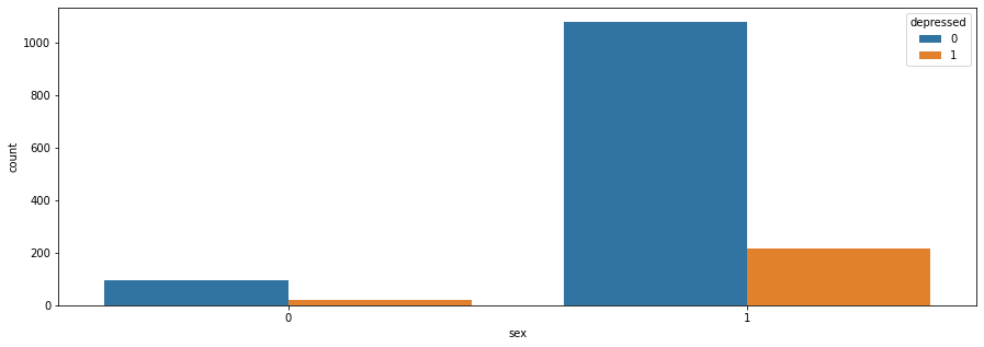
plt.figure(figsize=(15,5))
sns.countplot(x='sex',hue='depressed',data=df)
plt.show()

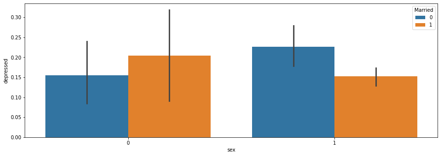
plt.figure(figsize=(15,5))
sns.barplot(x='sex',y='depressed',hue='Married',data=df)
plt.show()

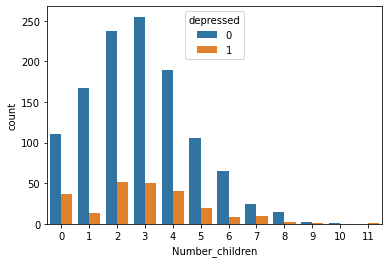
sns.countplot(x='Number_children', hue='depressed', data=df)

<AxesSubplot:xlabel='Number_children', ylabel='count'>

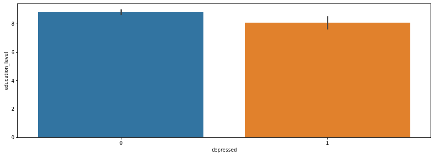
plt.figure(figsize=(15,5))
sns.barplot(x='depressed',y='education_level',data=df)
plt.show()

sel = alt.selection_single(fields=["depressed"])
c1= alt.Chart(df).mark_circle().encode(
    x="gained_asset",
    y="living_expenses",
    color=alt.Color('depressed')
)
c2= alt.Chart(df).mark_circle().encode(
    x="incoming_agricultural",
    y="lasting_investment",
    color=alt.Color('depressed')
)
c1&c2

Based on graphs, we can basically have an intuition about the dataset. Indicated by the graph, unmarried men are more likely to be depressed than married men and married women are more likely to be depressed than unmarried women. The people not despressed distributes normarlly as the number of children they have and people do not have children are more likely to be depressed.

Correlation¶

plt.subplots(figsize=(15,10)) 
sns.heatmap(df.corr(), annot = True, fmt = ".2f")
plt.show()

Here is the correlation matrix for all the predictor variables and response variable. Notice that the correlation between labor_primary and incoming-salary is 0.90. This indicates that people with high incoming-salary tend to also have high labor primary.

Train_Test_Split¶

socioecon_state = ['gained_asset','durable_asset', 'save_asset', 'living_expenses', 'other_expenses','incoming_agricultural', 'farm_expenses', 'lasting_investment']

X = df[socioecon_state]
y = df['depressed']

scaler = StandardScaler()
scaler.fit(X)

StandardScaler()

X_train, X_test, y_train, y_test = train_test_split(X,y, test_size = .2)

clf = KNeighborsClassifier()
clf.fit(X_train, y_train)

KNeighborsClassifier()

df['pred_depressed'] = pd.Series(clf.predict(X_test))

log_loss(df['depressed'], clf.predict_proba(X))

0.7256651995634845

The log loss is not that high hence the model is proper for predicting depression.

pred_depression_type = (df[['depressed', 'pred_depressed']]).copy()
pdt = pred_depression_type.value_counts(normalize=True)
pdt

depressed  pred_depressed
0          0.0               0.797101
1          0.0               0.184783
0          1.0               0.014493
1          1.0               0.003623
dtype: float64

Decision Tree¶

from sklearn.tree import DecisionTreeClassifier
from sklearn import tree

clf1 = DecisionTreeClassifier()

clf1.fit(df[socioecon_state],df["depressed"])

DecisionTreeClassifier()

clf1.score(df[socioecon_state],df["depressed"])

0.9460610361958836

fig = plt.figure(figsize=(200,100))
_ = tree.plot_tree(clf1, 
                   feature_names=clf1.feature_names_in_
                   )

Restrict the maximum depth and maximum number of leaf nodes by instantiating a new classifier

clf2 = DecisionTreeClassifier(max_depth=10, max_leaf_nodes=20)

clf2.fit(df[socioecon_state],df["depressed"])

DecisionTreeClassifier(max_depth=10, max_leaf_nodes=20)

clf2.score(df[socioecon_state],df["depressed"])

0.8523775727466288

fig = plt.figure(figsize=(200,100))
_ = tree.plot_tree(clf2, 
                   feature_names=clf2.feature_names_in_
                   )

Summary¶

In this project, I analyzed the datasets of rural residents’ depression. First, I created graphs to describe the distribution of depression regarding different factors. Some factors such as marriage, sex influence the probability of being depressed a lot and others such as education level do not impact the probability of being depressed a lot. Then, I presented the correlation between factors. Then, I used machine learning to analyze the dataset fitting data to see whether the numerical variables can predict being depressed. The last part is to build up decision tree for predicting depression and restricting the range of tree by setting up the max leaf nodes and max depth.

References¶

dataset source: https://www.kaggle.com/datasets/francispython/b-depression

Created in Deepnote

UC Irvine Math 10 S22

Depression Prediction

Contents