
Visualization in Python
Contents
Visualization in Python
Quick introduction to Matplotlib
Matplotlib is the most famous visualization library in Python. It has features that are very similar to the plotting features in Matlab. We actually won’t use Matplotlib much in Math 10 (we will use Altair more), so this will just be a short introduction.
There are a few different ways to use Matplotlib (which I think made it difficult for me to learn Matplotlib). The way we will present Matplotlib in Math 10 involves a little more writing but offers more flexibility and is more similar to typical Python code. Here is a relevant quote from the Matplotlib documentation:
We call methods that do the plotting directly from the Axes, which gives us much more flexibility and power in customizing our plot… In general, try to use the object-oriented interface over the pyplot interface.
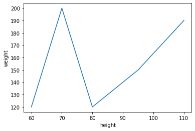
x = [70,95,60,110,80]
y = [200,150,120,190,120]
import matplotlib.pyplot as plt
For now don’t worry too much about what the line fig, ax = plt.subplots() is doing. You should imagine that plt.subplots() is returning two objects, one which we name fig and one which we name ax. The fig object is what shows the image, and the ax object is where we do the plotting. There is also a version where ax is an array of axes objects.
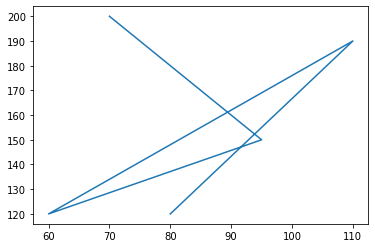
The line ax.plot(x,y) behaves very similarly to Matlab. We think of x as holding the x-coordinates and y as holding the y-coordinates. Matplotlib then connects the dots with straight lines, just like in Matlab.
fig, ax = plt.subplots()
ax.plot(x,y)
[<matplotlib.lines.Line2D at 0x7fb0ea103bd0>]
type(ax)
matplotlib.axes._subplots.AxesSubplot
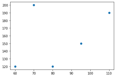
It’s very similar to make a scatter plot instead of a line plot.
fig, ax = plt.subplots()
ax.scatter(x,y)
<matplotlib.collections.PathCollection at 0x7fb0ea11dc90>

The fig object is what displays the image.
fig
Using NumPy and Matplotlib to plot cos(x)
Let’s plot y = cos(x) for x between 0 and 2pi. Our first attempt has lots of mistakes.
x1 = range(0,2*pi)
---------------------------------------------------------------------------
NameError                                 Traceback (most recent call last)
/var/folders/8j/gshrlmtn7dg4qtztj4d4t_w40000gn/T/ipykernel_14988/1058624340.py in <module>
----> 1 x1 = range(0,2*pi)

NameError: name 'pi' is not defined
import numpy as np
np.pi
3.141592653589793
Remember that range can only take integer arguments.
x1 = range(0,2*np.pi)
---------------------------------------------------------------------------
TypeError                                 Traceback (most recent call last)
/var/folders/8j/gshrlmtn7dg4qtztj4d4t_w40000gn/T/ipykernel_14988/86406984.py in <module>
----> 1 x1 = range(0,2*np.pi)

TypeError: 'float' object cannot be interpreted as an integer
NumPy provides a function very similar to range. The NumPy version is called arange, and it accepts float arguments.
x1 = np.arange(0,2*np.pi)
Python’s range makes objects of type range. NumPy’s arange makes objects of type numpy.ndarray, which is the most common data type in NumPy.
type(x1)
numpy.ndarray
Now let’s try to make the y-coordinates.
y1 = cos(x1)
---------------------------------------------------------------------------
NameError                                 Traceback (most recent call last)
/var/folders/8j/gshrlmtn7dg4qtztj4d4t_w40000gn/T/ipykernel_14988/1263318031.py in <module>
----> 1 y1 = cos(x1)

NameError: name 'cos' is not defined
y1 = np.cos(x1)
fig, ax = plt.subplots()
ax.plot(x1,y1)
[<matplotlib.lines.Line2D at 0x7fb0d8f3e490>]
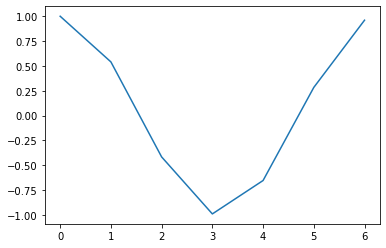
It doesn’t look very good because the step size is too big. By default, arange (and range) uses a step size of 1.
x1
array([0., 1., 2., 3., 4., 5., 6.])
x1.shape
(7,)
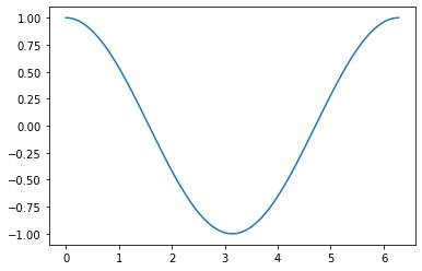
Here we use a step size of 0.01.
x2 = np.arange(0,2*np.pi,0.01)
y2 = np.cos(x2)
fig, ax = plt.subplots()
ax.plot(x2,y2)
[<matplotlib.lines.Line2D at 0x7fb0d9028390>]
Plotting based on the Grammar of Graphics
Here we will introduce three more plotting libraries: Altair (the most important for us in Math 10), Seaborn, and Plotly. These three libraries are very similar to each other (not so similar to Matplotlib, although Seaborn is built on top of Matplotlib), and I believe all three are based on a notion called the Grammar of Graphics. (Here is the book The Grammar of Graphics, which is freely available to download from on campus or using VPN.)
Here is the basic setup:
We have a pandas DataFrame, and each row in the DataFrame corresponds to one observation (or one data point).
Columns in the DataFrame correspond to different variables.
To produce the visualizations, we encode different columns from the DataFrame into visual properties of the chart.
import pandas as pd
Making a pandas DataFrame using our same x and y lists from above.
x
[70, 95, 60, 110, 80]
y
[200, 150, 120, 190, 120]
df = pd.DataFrame({"height":x, "weight":y})
df
| height | weight | |
|---|---|---|
| 0 | 70 | 200 |
| 1 | 95 | 150 |
| 2 | 60 | 120 |
| 3 | 110 | 190 |
| 4 | 80 | 120 |
df.columns
Index(['height', 'weight'], dtype='object')
Let’s first plot this data using Seaborn, which I think is the most famous member of this family of plotting libraries.
import seaborn as sns
Notice that we specify the pandas DataFrame which holds the data, as well as which column to use for the x-coordinates and which column to use for y-coordinates. By default, Seaborn sorts the data so that the x-coordinates are increasing (that’s why the lines do not cross each other here).
sns.lineplot(
    data=df,
    x="height",
    y="weight"
)
<AxesSubplot:xlabel='height', ylabel='weight'>
The term data above is what’s called a keyword argument. It gets temporarily given the value df, but that only happens locally, we do not have any record of that ourselves.
data
---------------------------------------------------------------------------
NameError                                 Traceback (most recent call last)
/var/folders/8j/gshrlmtn7dg4qtztj4d4t_w40000gn/T/ipykernel_14988/391604064.py in <module>
----> 1 data

NameError: name 'data' is not defined
Here is the Plotly version of the same plot.
import plotly.express as px
This is very similar. It uses the keyword argument data_frame instead of data, and it does not order the x-values, but otherwise it is quite similar.
px.line(
    data_frame=df,
    x="height",
    y="weight"
)
Here is the Altair version of the same plot. Altair is the plotting library we will use most often in Math 10. The syntax is a little different from the Seaborn and Plotly syntax. It is worth practicing with this Altair syntax until you get comfortable with it.
import altair as alt
alt.Chart(data=df).mark_line().encode(
    x="height",
    y="weight"
)
If we want to change from a line plot to a scatter plot, in Altair, we change mark_line to mark_circle.
alt.Chart(data=df).mark_circle().encode(
    x="height",
    y="weight"
)
Let’s see how to change the domain shown on the x-axis. As an intermediate step, we give the longer version of the same code as above. We change x="height" to x=alt.X("height"). So far, this does not change the chart.
alt.Chart(data=df).mark_circle().encode(
    x=alt.X("height"),
    y="weight"
)
Now we add a new keyword argument inside alt.X which specifies that the x-values should be displayed between -100 and 500.
alt.Chart(data=df).mark_circle().encode(
    x=alt.X("height", scale=alt.Scale(domain=(-100,500))),
    y="weight"
)
If instead you want Altair to choose for you, but not force 0 to be included, you can specify zero=False. Here it zooms in as much as possible. (For now it is only changing the x-values, not the y-values, because we are only using alt.X, not alt.Y.)
alt.Chart(data=df).mark_circle().encode(
    x=alt.X("height", scale=alt.Scale(zero=False)),
    y="weight"
)
Let’s recall what data is in df.
df
| height | weight | |
|---|---|---|
| 0 | 70 | 200 |
| 1 | 95 | 150 |
| 2 | 60 | 120 |
| 3 | 110 | 190 |
| 4 | 80 | 120 |
Here is a method for creating a new column in a DataFrame. The most important thing is that the number of values we provide is equal to the number of rows. That’s why we give 5 state names in this case.
df["state"] = ["California","California","Oregon","Nevada","Arizona"]
df
| height | weight | state | |
|---|---|---|---|
| 0 | 70 | 200 | California |
| 1 | 95 | 150 | California |
| 2 | 60 | 120 | Oregon |
| 3 | 110 | 190 | Nevada |
| 4 | 80 | 120 | Arizona |
Let’s add one more column, containing floats.
df["GPA"] = [1.5, 2.4, 4, 3.5, 4.7]
df
| height | weight | state | GPA | |
|---|---|---|---|---|
| 0 | 70 | 200 | California | 1.5 |
| 1 | 95 | 150 | California | 2.4 |
| 2 | 60 | 120 | Oregon | 4.0 |
| 3 | 110 | 190 | Nevada | 3.5 |
| 4 | 80 | 120 | Arizona | 4.7 |
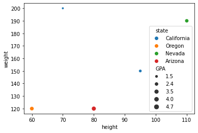
Here we encode the “state” column into the color of the chart, and we encode the “GPA” column into the size of the points.
alt.Chart(data=df).mark_circle().encode(
    x=alt.X("height", scale=alt.Scale(zero=False)),
    y="weight",
    color="state",
    size="GPA"
)
Everything works very similarly in Seaborn and in Plotly. Here is the Seaborn version.
sns.scatterplot(
    data=df,
    x="height",
    y="weight",
    hue="state",
    size="GPA"
)
<AxesSubplot:xlabel='height', ylabel='weight'>
Here is the Plotly version.
px.scatter(
    data_frame=df,
    x="height",
    y="weight",
    color="state",
    size="GPA"
)
Let’s access the row at index 2 of the DataFrame. Using df[2] doesn’t work; if we use df[2], pandas is looking for a column with the name 2.
df[2]
---------------------------------------------------------------------------
KeyError                                  Traceback (most recent call last)
~/miniconda3/envs/math10s22/lib/python3.7/site-packages/pandas/core/indexes/base.py in get_loc(self, key, method, tolerance)
   3360             try:
-> 3361                 return self._engine.get_loc(casted_key)
   3362             except KeyError as err:

~/miniconda3/envs/math10s22/lib/python3.7/site-packages/pandas/_libs/index.pyx in pandas._libs.index.IndexEngine.get_loc()

~/miniconda3/envs/math10s22/lib/python3.7/site-packages/pandas/_libs/index.pyx in pandas._libs.index.IndexEngine.get_loc()

pandas/_libs/hashtable_class_helper.pxi in pandas._libs.hashtable.PyObjectHashTable.get_item()

pandas/_libs/hashtable_class_helper.pxi in pandas._libs.hashtable.PyObjectHashTable.get_item()

KeyError: 2

The above exception was the direct cause of the following exception:

KeyError                                  Traceback (most recent call last)
/var/folders/8j/gshrlmtn7dg4qtztj4d4t_w40000gn/T/ipykernel_14988/2772902488.py in <module>
----> 1 df[2]

~/miniconda3/envs/math10s22/lib/python3.7/site-packages/pandas/core/frame.py in __getitem__(self, key)
   3456             if self.columns.nlevels > 1:
   3457                 return self._getitem_multilevel(key)
-> 3458             indexer = self.columns.get_loc(key)
   3459             if is_integer(indexer):
   3460                 indexer = [indexer]

~/miniconda3/envs/math10s22/lib/python3.7/site-packages/pandas/core/indexes/base.py in get_loc(self, key, method, tolerance)
   3361                 return self._engine.get_loc(casted_key)
   3362             except KeyError as err:
-> 3363                 raise KeyError(key) from err
   3364
   3365         if is_scalar(key) and isna(key) and not self.hasnans:

KeyError: 2
Here is the right way to find the row at index 2.
We think of each row as corresponding to one observation. In this case, each row could correspond to one person. It’s worth looking at the data in this row, and looking back at the three plots from Altair, Seaborn, and Plotly, and seeing how this data is encoded in one of the 5 data points from these charts. The point is at coordinates (60,120), it is colored according to the state being “Oregon”, and the size corresponds to the GPA value.
df.iloc[2]
height        60
weight       120
state     Oregon
GPA          4.0
Name: 2, dtype: object
If you try to use px.scatter(data=...) you will get an error. It needs to be px.scatter(data_frame=...). This data_frame is a keyword argument to the scatter function, as you can see at the beginning of the documentation.
help(px.scatter)
Help on function scatter in module plotly.express._chart_types:

scatter(data_frame=None, x=None, y=None, color=None, symbol=None, size=None, hover_name=None, hover_data=None, custom_data=None, text=None, facet_row=None, facet_col=None, facet_col_wrap=0, facet_row_spacing=None, facet_col_spacing=None, error_x=None, error_x_minus=None, error_y=None, error_y_minus=None, animation_frame=None, animation_group=None, category_orders=None, labels=None, orientation=None, color_discrete_sequence=None, color_discrete_map=None, color_continuous_scale=None, range_color=None, color_continuous_midpoint=None, symbol_sequence=None, symbol_map=None, opacity=None, size_max=None, marginal_x=None, marginal_y=None, trendline=None, trendline_options=None, trendline_color_override=None, trendline_scope='trace', log_x=False, log_y=False, range_x=None, range_y=None, render_mode='auto', title=None, template=None, width=None, height=None)
        In a scatter plot, each row of `data_frame` is represented by a symbol
        mark in 2D space.

    Parameters
    ----------
    data_frame: DataFrame or array-like or dict
        This argument needs to be passed for column names (and not keyword
        names) to be used. Array-like and dict are tranformed internally to a
        pandas DataFrame. Optional: if missing, a DataFrame gets constructed
        under the hood using the other arguments.
    x: str or int or Series or array-like
        Either a name of a column in `data_frame`, or a pandas Series or
        array_like object. Values from this column or array_like are used to
        position marks along the x axis in cartesian coordinates. Either `x` or
        `y` can optionally be a list of column references or array_likes,  in
        which case the data will be treated as if it were 'wide' rather than
        'long'.
    y: str or int or Series or array-like
        Either a name of a column in `data_frame`, or a pandas Series or
        array_like object. Values from this column or array_like are used to
        position marks along the y axis in cartesian coordinates. Either `x` or
        `y` can optionally be a list of column references or array_likes,  in
        which case the data will be treated as if it were 'wide' rather than
        'long'.
    color: str or int or Series or array-like
        Either a name of a column in `data_frame`, or a pandas Series or
        array_like object. Values from this column or array_like are used to
        assign color to marks.
    symbol: str or int or Series or array-like
        Either a name of a column in `data_frame`, or a pandas Series or
        array_like object. Values from this column or array_like are used to
        assign symbols to marks.
    size: str or int or Series or array-like
        Either a name of a column in `data_frame`, or a pandas Series or
        array_like object. Values from this column or array_like are used to
        assign mark sizes.
    hover_name: str or int or Series or array-like
        Either a name of a column in `data_frame`, or a pandas Series or
        array_like object. Values from this column or array_like appear in bold
        in the hover tooltip.
    hover_data: list of str or int, or Series or array-like, or dict
        Either a list of names of columns in `data_frame`, or pandas Series, or
        array_like objects or a dict with column names as keys, with values
        True (for default formatting) False (in order to remove this column
        from hover information), or a formatting string, for example ':.3f' or
        '|%a' or list-like data to appear in the hover tooltip or tuples with a
        bool or formatting string as first element, and list-like data to
        appear in hover as second element Values from these columns appear as
        extra data in the hover tooltip.
    custom_data: list of str or int, or Series or array-like
        Either names of columns in `data_frame`, or pandas Series, or
        array_like objects Values from these columns are extra data, to be used
        in widgets or Dash callbacks for example. This data is not user-visible
        but is included in events emitted by the figure (lasso selection etc.)
    text: str or int or Series or array-like
        Either a name of a column in `data_frame`, or a pandas Series or
        array_like object. Values from this column or array_like appear in the
        figure as text labels.
    facet_row: str or int or Series or array-like
        Either a name of a column in `data_frame`, or a pandas Series or
        array_like object. Values from this column or array_like are used to
        assign marks to facetted subplots in the vertical direction.
    facet_col: str or int or Series or array-like
        Either a name of a column in `data_frame`, or a pandas Series or
        array_like object. Values from this column or array_like are used to
        assign marks to facetted subplots in the horizontal direction.
    facet_col_wrap: int
        Maximum number of facet columns. Wraps the column variable at this
        width, so that the column facets span multiple rows. Ignored if 0, and
        forced to 0 if `facet_row` or a `marginal` is set.
    facet_row_spacing: float between 0 and 1
        Spacing between facet rows, in paper units. Default is 0.03 or 0.0.7
        when facet_col_wrap is used.
    facet_col_spacing: float between 0 and 1
        Spacing between facet columns, in paper units Default is 0.02.
    error_x: str or int or Series or array-like
        Either a name of a column in `data_frame`, or a pandas Series or
        array_like object. Values from this column or array_like are used to
        size x-axis error bars. If `error_x_minus` is `None`, error bars will
        be symmetrical, otherwise `error_x` is used for the positive direction
        only.
    error_x_minus: str or int or Series or array-like
        Either a name of a column in `data_frame`, or a pandas Series or
        array_like object. Values from this column or array_like are used to
        size x-axis error bars in the negative direction. Ignored if `error_x`
        is `None`.
    error_y: str or int or Series or array-like
        Either a name of a column in `data_frame`, or a pandas Series or
        array_like object. Values from this column or array_like are used to
        size y-axis error bars. If `error_y_minus` is `None`, error bars will
        be symmetrical, otherwise `error_y` is used for the positive direction
        only.
    error_y_minus: str or int or Series or array-like
        Either a name of a column in `data_frame`, or a pandas Series or
        array_like object. Values from this column or array_like are used to
        size y-axis error bars in the negative direction. Ignored if `error_y`
        is `None`.
    animation_frame: str or int or Series or array-like
        Either a name of a column in `data_frame`, or a pandas Series or
        array_like object. Values from this column or array_like are used to
        assign marks to animation frames.
    animation_group: str or int or Series or array-like
        Either a name of a column in `data_frame`, or a pandas Series or
        array_like object. Values from this column or array_like are used to
        provide object-constancy across animation frames: rows with matching
        `animation_group`s will be treated as if they describe the same object
        in each frame.
    category_orders: dict with str keys and list of str values (default `{}`)
        By default, in Python 3.6+, the order of categorical values in axes,
        legends and facets depends on the order in which these values are first
        encountered in `data_frame` (and no order is guaranteed by default in
        Python below 3.6). This parameter is used to force a specific ordering
        of values per column. The keys of this dict should correspond to column
        names, and the values should be lists of strings corresponding to the
        specific display order desired.
    labels: dict with str keys and str values (default `{}`)
        By default, column names are used in the figure for axis titles, legend
        entries and hovers. This parameter allows this to be overridden. The
        keys of this dict should correspond to column names, and the values
        should correspond to the desired label to be displayed.
    orientation: str, one of `'h'` for horizontal or `'v'` for vertical.
        (default `'v'` if `x` and `y` are provided and both continous or both
        categorical,  otherwise `'v'`(`'h'`) if `x`(`y`) is categorical and
        `y`(`x`) is continuous,  otherwise `'v'`(`'h'`) if only `x`(`y`) is
        provided)
    color_discrete_sequence: list of str
        Strings should define valid CSS-colors. When `color` is set and the
        values in the corresponding column are not numeric, values in that
        column are assigned colors by cycling through `color_discrete_sequence`
        in the order described in `category_orders`, unless the value of
        `color` is a key in `color_discrete_map`. Various useful color
        sequences are available in the `plotly.express.colors` submodules,
        specifically `plotly.express.colors.qualitative`.
    color_discrete_map: dict with str keys and str values (default `{}`)
        String values should define valid CSS-colors Used to override
        `color_discrete_sequence` to assign a specific colors to marks
        corresponding with specific values. Keys in `color_discrete_map` should
        be values in the column denoted by `color`. Alternatively, if the
        values of `color` are valid colors, the string `'identity'` may be
        passed to cause them to be used directly.
    color_continuous_scale: list of str
        Strings should define valid CSS-colors This list is used to build a
        continuous color scale when the column denoted by `color` contains
        numeric data. Various useful color scales are available in the
        `plotly.express.colors` submodules, specifically
        `plotly.express.colors.sequential`, `plotly.express.colors.diverging`
        and `plotly.express.colors.cyclical`.
    range_color: list of two numbers
        If provided, overrides auto-scaling on the continuous color scale.
    color_continuous_midpoint: number (default `None`)
        If set, computes the bounds of the continuous color scale to have the
        desired midpoint. Setting this value is recommended when using
        `plotly.express.colors.diverging` color scales as the inputs to
        `color_continuous_scale`.
    symbol_sequence: list of str
        Strings should define valid plotly.js symbols. When `symbol` is set,
        values in that column are assigned symbols by cycling through
        `symbol_sequence` in the order described in `category_orders`, unless
        the value of `symbol` is a key in `symbol_map`.
    symbol_map: dict with str keys and str values (default `{}`)
        String values should define plotly.js symbols Used to override
        `symbol_sequence` to assign a specific symbols to marks corresponding
        with specific values. Keys in `symbol_map` should be values in the
        column denoted by `symbol`. Alternatively, if the values of `symbol`
        are valid symbol names, the string `'identity'` may be passed to cause
        them to be used directly.
    opacity: float
        Value between 0 and 1. Sets the opacity for markers.
    size_max: int (default `20`)
        Set the maximum mark size when using `size`.
    marginal_x: str
        One of `'rug'`, `'box'`, `'violin'`, or `'histogram'`. If set, a
        horizontal subplot is drawn above the main plot, visualizing the
        x-distribution.
    marginal_y: str
        One of `'rug'`, `'box'`, `'violin'`, or `'histogram'`. If set, a
        vertical subplot is drawn to the right of the main plot, visualizing
        the y-distribution.
    trendline: str
        One of `'ols'`, `'lowess'`, `'rolling'`, `'expanding'` or `'ewm'`. If
        `'ols'`, an Ordinary Least Squares regression line will be drawn for
        each discrete-color/symbol group. If `'lowess`', a Locally Weighted
        Scatterplot Smoothing line will be drawn for each discrete-color/symbol
        group. If `'rolling`', a Rolling (e.g. rolling average, rolling median)
        line will be drawn for each discrete-color/symbol group. If
        `'expanding`', an Expanding (e.g. expanding average, expanding sum)
        line will be drawn for each discrete-color/symbol group. If `'ewm`', an
        Exponentially Weighted Moment (e.g. exponentially-weighted moving
        average) line will be drawn for each discrete-color/symbol group. See
        the docstrings for the functions in
        `plotly.express.trendline_functions` for more details on these
        functions and how to configure them with the `trendline_options`
        argument.
    trendline_options: dict
        Options passed as the first argument to the function from
        `plotly.express.trendline_functions`  named in the `trendline`
        argument.
    trendline_color_override: str
        Valid CSS color. If provided, and if `trendline` is set, all trendlines
        will be drawn in this color rather than in the same color as the traces
        from which they draw their inputs.
    trendline_scope: str (one of `'trace'` or `'overall'`, default `'trace'`)
        If `'trace'`, then one trendline is drawn per trace (i.e. per color,
        symbol, facet, animation frame etc) and if `'overall'` then one
        trendline is computed for the entire dataset, and replicated across all
        facets.
    log_x: boolean (default `False`)
        If `True`, the x-axis is log-scaled in cartesian coordinates.
    log_y: boolean (default `False`)
        If `True`, the y-axis is log-scaled in cartesian coordinates.
    range_x: list of two numbers
        If provided, overrides auto-scaling on the x-axis in cartesian
        coordinates.
    range_y: list of two numbers
        If provided, overrides auto-scaling on the y-axis in cartesian
        coordinates.
    render_mode: str
        One of `'auto'`, `'svg'` or `'webgl'`, default `'auto'` Controls the
        browser API used to draw marks. `'svg`' is appropriate for figures of
        less than 1000 data points, and will allow for fully-vectorized output.
        `'webgl'` is likely necessary for acceptable performance above 1000
        points but rasterizes part of the output.  `'auto'` uses heuristics to
        choose the mode.
    title: str
        The figure title.
    template: str or dict or plotly.graph_objects.layout.Template instance
        The figure template name (must be a key in plotly.io.templates) or
        definition.
    width: int (default `None`)
        The figure width in pixels.
    height: int (default `None`)
        The figure height in pixels.

    Returns
    -------
        plotly.graph_objects.Figure