
Customer Personality Analysis
Contents
Customer Personality Analysis#
Author: Aner Huang
Course Project, UC Irvine, Math 10, F22
Introduction#
For this project, I chose “Customer Personality Analysis.” It is about the detailed analysis of a company’s ideal customers. It helps a business to better understand its customers and makes it easier for them to modify products according to the specific needs, behaviors and concerns of different types of customers.Customer personality analysis helps a business to modify its product based on its target customers from different types of customer segments. Since it contains a lot of factor to analyze, I only focus on the catalog of “people”, including “Age”, “Income”, “Education”,and “Marital_status”.
Section 1: Overview and Clean Dataset#
To begin, I will firstly import some packages that I am going to use in this project and analysis.
Then, I will load my dataset and show some basic information of my dataset.
import pandas as pd
import numpy as np
# Read the dataset
df=pd.read_csv("Costomer_Personality.csv")
df
| ID | Year_Birth | Education | Marital_Status | Income | Kidhome | Teenhome | Dt_Customer | Recency | MntWines | ... | NumWebVisitsMonth | AcceptedCmp3 | AcceptedCmp4 | AcceptedCmp5 | AcceptedCmp1 | AcceptedCmp2 | Complain | Z_CostContact | Z_Revenue | Response | |
|---|---|---|---|---|---|---|---|---|---|---|---|---|---|---|---|---|---|---|---|---|---|
| 0 | 5524 | 1957 | Graduation | Single | 58138.0 | 0 | 0 | 04-09-2012 | 58 | 635 | ... | 7 | 0 | 0 | 0 | 0 | 0 | 0 | 3 | 11 | 1 |
| 1 | 2174 | 1954 | Graduation | Single | 46344.0 | 1 | 1 | 08-03-2014 | 38 | 11 | ... | 5 | 0 | 0 | 0 | 0 | 0 | 0 | 3 | 11 | 0 |
| 2 | 4141 | 1965 | Graduation | Together | 71613.0 | 0 | 0 | 21-08-2013 | 26 | 426 | ... | 4 | 0 | 0 | 0 | 0 | 0 | 0 | 3 | 11 | 0 |
| 3 | 6182 | 1984 | Graduation | Together | 26646.0 | 1 | 0 | 10-02-2014 | 26 | 11 | ... | 6 | 0 | 0 | 0 | 0 | 0 | 0 | 3 | 11 | 0 |
| 4 | 5324 | 1981 | PhD | Married | 58293.0 | 1 | 0 | 19-01-2014 | 94 | 173 | ... | 5 | 0 | 0 | 0 | 0 | 0 | 0 | 3 | 11 | 0 |
| ... | ... | ... | ... | ... | ... | ... | ... | ... | ... | ... | ... | ... | ... | ... | ... | ... | ... | ... | ... | ... | ... |
| 2235 | 10870 | 1967 | Graduation | Married | 61223.0 | 0 | 1 | 13-06-2013 | 46 | 709 | ... | 5 | 0 | 0 | 0 | 0 | 0 | 0 | 3 | 11 | 0 |
| 2236 | 4001 | 1946 | PhD | Together | 64014.0 | 2 | 1 | 10-06-2014 | 56 | 406 | ... | 7 | 0 | 0 | 0 | 1 | 0 | 0 | 3 | 11 | 0 |
| 2237 | 7270 | 1981 | Graduation | Divorced | 56981.0 | 0 | 0 | 25-01-2014 | 91 | 908 | ... | 6 | 0 | 1 | 0 | 0 | 0 | 0 | 3 | 11 | 0 |
| 2238 | 8235 | 1956 | Master | Together | 69245.0 | 0 | 1 | 24-01-2014 | 8 | 428 | ... | 3 | 0 | 0 | 0 | 0 | 0 | 0 | 3 | 11 | 0 |
| 2239 | 9405 | 1954 | PhD | Married | 52869.0 | 1 | 1 | 15-10-2012 | 40 | 84 | ... | 7 | 0 | 0 | 0 | 0 | 0 | 0 | 3 | 11 | 1 |
2240 rows × 29 columns
# Dimension of dataset
df.shape
(2240, 29)
# Counting numbers of missing values in each column
df.isna().sum()
ID                      0
Year_Birth              0
Education               0
Marital_Status          0
Income                 24
Kidhome                 0
Teenhome                0
Dt_Customer             0
Recency                 0
MntWines                0
MntFruits               0
MntMeatProducts         0
MntFishProducts         0
MntSweetProducts        0
MntGoldProds            0
NumDealsPurchases       0
NumWebPurchases         0
NumCatalogPurchases     0
NumStorePurchases       0
NumWebVisitsMonth       0
AcceptedCmp3            0
AcceptedCmp4            0
AcceptedCmp5            0
AcceptedCmp1            0
AcceptedCmp2            0
Complain                0
Z_CostContact           0
Z_Revenue               0
Response                0
dtype: int64
We can see that we have 24 missing values in the colume “Income”, we can fill these bad datas as the median of the colume of “Income” using
fillna
df['Income']=df['Income'].fillna(df['Income'].median())
Section1.1: A Brief Introduction of Dataset#
In order for us to better analyze this dataset, I will make a better clear names for those columns that have an ambiguious name and I will also clarity the meaning of each columns for people to understand.
For the following, I normalize the dataset by using the method of
rename.
# List out all the names of columns
df.columns
Index(['ID', 'Year_Birth', 'Education', 'Marital_Status', 'Income', 'Kidhome',
       'Teenhome', 'Dt_Customer', 'Recency', 'MntWines', 'MntFruits',
       'MntMeatProducts', 'MntFishProducts', 'MntSweetProducts',
       'MntGoldProds', 'NumDealsPurchases', 'NumWebPurchases',
       'NumCatalogPurchases', 'NumStorePurchases', 'NumWebVisitsMonth',
       'AcceptedCmp3', 'AcceptedCmp4', 'AcceptedCmp5', 'AcceptedCmp1',
       'AcceptedCmp2', 'Complain', 'Z_CostContact', 'Z_Revenue', 'Response'],
      dtype='object')
# Normalizing Dataset
df.rename({"Dt_Customer ":"Date","MntWines":"Wines","MntFruits":"Fruits","MntMeatProducts":"Meat","MntFishProducts":"Fish","MntSweetProducts":"Sweet","MntGoldProds":"Gold","NumDealsPurchases":"Deals","NumWebPurchases":"Web","NumCatalogPurchases":"Catalog","NumWebVisitsMonth":"WebVisit"},axis=1,inplace=True)
Create another feature “Total” indicating the total amount spent by the customer in various categories over the span of two years.
Classify the objects in “Marital_Status” to extract the living situation of couples.
Dropping some of the redundant features and other features that I am not going to analyze in this project using
drop.
df["Total"] = df["Wines"]+df["Fruits"]+df["Meat"]+df["Fish"]+df["Sweet"]+df["Gold"]
df['Marital_Status'] = df['Marital_Status'].replace({'Married':'Relationship', 'Together':'Relationship','Divorced':'Alone','Widow':'Alone','YOLO':'Alone', 'Absurd':'Alone'})
to_drop = ["Kidhome","Teenhome", "Z_CostContact", "Z_Revenue"]
df = df.drop(to_drop, axis=1)
Brief Introduction of Columns:
People: ID: Customer’s unique identifier Year_Birth: Customer’s birth year Education: Customer’s education level Marital_Status: Customer’s marital status Income: Customer’s yearly household income Kidhome: Number of children in customer’s household Teenhome: Number of teenagers in customer’s household Date: Date of customer’s enrollment with the company Recency: Number of days since customer’s last purchase Complain: 1 if the customer complained in the last 2 years, 0 otherwise
Products: Wines: Amount spent on wine in last 2 years Fruits: Amount spent on fruits in last 2 years Meat: Amount spent on meat in last 2 years Fish: Amount spent on fish in last 2 years Sweet: Amount spent on sweets in last 2 years Gold: Amount spent on gold in last 2 years
Promotion: Deals: Number of purchases made with a discount AcceptedCmp1: 1 if customer accepted the offer in the 1st campaign, 0 otherwise AcceptedCmp2: 1 if customer accepted the offer in the 2nd campaign, 0 otherwise AcceptedCmp3: 1 if customer accepted the offer in the 3rd campaign, 0 otherwise AcceptedCmp4: 1 if customer accepted the offer in the 4th campaign, 0 otherwise AcceptedCmp5: 1 if customer accepted the offer in the 5th campaign, 0 otherwise Response: 1 if customer accepted the offer in the last campaign, 0 otherwise
Place: Web: Number of purchases made through the company’s website Catalog: Number of purchases made using a catalogue Store: Number of purchases made directly in stores WebVisits: Number of visits to company’s website in the last month
# Description of Data
df.describe()
| ID | Year_Birth | Income | Recency | Wines | Fruits | Meat | Fish | Sweet | Gold | ... | NumStorePurchases | WebVisit | AcceptedCmp3 | AcceptedCmp4 | AcceptedCmp5 | AcceptedCmp1 | AcceptedCmp2 | Complain | Response | Total | |
|---|---|---|---|---|---|---|---|---|---|---|---|---|---|---|---|---|---|---|---|---|---|
| count | 2240.000000 | 2240.000000 | 2240.000000 | 2240.000000 | 2240.000000 | 2240.000000 | 2240.000000 | 2240.000000 | 2240.000000 | 2240.000000 | ... | 2240.000000 | 2240.000000 | 2240.000000 | 2240.000000 | 2240.000000 | 2240.000000 | 2240.000000 | 2240.000000 | 2240.000000 | 2240.000000 |
| mean | 5592.159821 | 1968.805804 | 52237.975446 | 49.109375 | 303.935714 | 26.302232 | 166.950000 | 37.525446 | 27.062946 | 44.021875 | ... | 5.790179 | 5.316518 | 0.072768 | 0.074554 | 0.072768 | 0.064286 | 0.013393 | 0.009375 | 0.149107 | 605.798214 |
| std | 3246.662198 | 11.984069 | 25037.955891 | 28.962453 | 336.597393 | 39.773434 | 225.715373 | 54.628979 | 41.280498 | 52.167439 | ... | 3.250958 | 2.426645 | 0.259813 | 0.262728 | 0.259813 | 0.245316 | 0.114976 | 0.096391 | 0.356274 | 602.249288 |
| min | 0.000000 | 1893.000000 | 1730.000000 | 0.000000 | 0.000000 | 0.000000 | 0.000000 | 0.000000 | 0.000000 | 0.000000 | ... | 0.000000 | 0.000000 | 0.000000 | 0.000000 | 0.000000 | 0.000000 | 0.000000 | 0.000000 | 0.000000 | 5.000000 |
| 25% | 2828.250000 | 1959.000000 | 35538.750000 | 24.000000 | 23.750000 | 1.000000 | 16.000000 | 3.000000 | 1.000000 | 9.000000 | ... | 3.000000 | 3.000000 | 0.000000 | 0.000000 | 0.000000 | 0.000000 | 0.000000 | 0.000000 | 0.000000 | 68.750000 |
| 50% | 5458.500000 | 1970.000000 | 51381.500000 | 49.000000 | 173.500000 | 8.000000 | 67.000000 | 12.000000 | 8.000000 | 24.000000 | ... | 5.000000 | 6.000000 | 0.000000 | 0.000000 | 0.000000 | 0.000000 | 0.000000 | 0.000000 | 0.000000 | 396.000000 |
| 75% | 8427.750000 | 1977.000000 | 68289.750000 | 74.000000 | 504.250000 | 33.000000 | 232.000000 | 50.000000 | 33.000000 | 56.000000 | ... | 8.000000 | 7.000000 | 0.000000 | 0.000000 | 0.000000 | 0.000000 | 0.000000 | 0.000000 | 0.000000 | 1045.500000 |
| max | 11191.000000 | 1996.000000 | 666666.000000 | 99.000000 | 1493.000000 | 199.000000 | 1725.000000 | 259.000000 | 263.000000 | 362.000000 | ... | 13.000000 | 20.000000 | 1.000000 | 1.000000 | 1.000000 | 1.000000 | 1.000000 | 1.000000 | 1.000000 | 2525.000000 |
8 rows × 23 columns
Section2: The Relationships between Customer’s life status and Total Amount of Purchase#
2.1. Generation#
For this section, I am interested in analyzing the relationship between Costomer’s Age and the total purchases they made.
For total purchases, I will need to make a new column contains the total number they purchased in the last two year by adding up the amount of Wines, Fruits, Meat, Fish, Sweet, and Gold.
I will also create a new column “Age” represents customer’s age also a “generation” column represents customer’s generation and narrow the range to the age under 80, thus we will also have generation 2-7.
I will also include charts about the distribution of different generation.
#Current year minus the year of birth will be the age of customers
df["Age"] = 2022-df["Year_Birth"]
df = df[df["Age"]<80] #Narrow my age range
Using
mapmethod to create a new column called “Generation” to specify different age group.But first, I would need to make the “Age” column becomes ‘str’ instead of ‘int’, so the numbers in the “Age” column does not have any numerical meaning, instead it will represents the age group.
df["Age"]=df["Age"].apply(str)
df["Generation"] = df["Age"].map(lambda x: x[:1])
df.groupby("Generation", sort=True).mean()
| ID | Year_Birth | Income | Recency | Wines | Fruits | Meat | Fish | Sweet | Gold | ... | NumStorePurchases | WebVisit | AcceptedCmp3 | AcceptedCmp4 | AcceptedCmp5 | AcceptedCmp1 | AcceptedCmp2 | Complain | Response | Total | |
|---|---|---|---|---|---|---|---|---|---|---|---|---|---|---|---|---|---|---|---|---|---|
| Generation | |||||||||||||||||||||
| 2 | 6322.066667 | 1994.266667 | 63576.866667 | 48.466667 | 357.133333 | 43.266667 | 341.800000 | 93.733333 | 46.066667 | 69.466667 | ... | 6.533333 | 3.533333 | 0.133333 | 0.066667 | 0.266667 | 0.133333 | 0.066667 | 0.066667 | 0.333333 | 951.466667 |
| 3 | 5768.597902 | 1986.580420 | 44734.256993 | 48.597902 | 236.062937 | 27.716783 | 177.961538 | 33.734266 | 28.678322 | 42.465035 | ... | 5.174825 | 5.541958 | 0.104895 | 0.045455 | 0.108392 | 0.090909 | 0.010490 | 0.010490 | 0.185315 | 546.618881 |
| 4 | 5525.400000 | 1976.875806 | 49610.597581 | 48.641935 | 243.335484 | 23.079032 | 146.127419 | 34.843548 | 24.658065 | 37.869355 | ... | 5.350000 | 5.622581 | 0.087097 | 0.053226 | 0.064516 | 0.053226 | 0.006452 | 0.009677 | 0.135484 | 509.912903 |
| 5 | 5452.600000 | 1968.069355 | 51744.570161 | 49.272581 | 309.001613 | 26.140323 | 152.582258 | 34.350000 | 25.474194 | 44.366129 | ... | 5.746774 | 5.554839 | 0.062903 | 0.083871 | 0.051613 | 0.043548 | 0.016129 | 0.001613 | 0.145161 | 591.914516 |
| 6 | 5710.436559 | 1957.479570 | 57179.921505 | 50.094624 | 374.451613 | 27.636559 | 183.632258 | 42.415054 | 29.167742 | 47.741935 | ... | 6.372043 | 4.888172 | 0.055914 | 0.101075 | 0.070968 | 0.079570 | 0.023656 | 0.012903 | 0.141935 | 705.045161 |
| 7 | 5617.890830 | 1949.266376 | 59004.475983 | 48.240175 | 389.384279 | 29.615721 | 201.122271 | 44.572052 | 30.633188 | 52.218341 | ... | 6.689956 | 4.589520 | 0.052402 | 0.091703 | 0.091703 | 0.082969 | 0.004367 | 0.013100 | 0.157205 | 747.545852 |
6 rows × 23 columns
df["Generation"].value_counts()
4    620
5    620
6    465
3    286
7    229
2     15
Name: Generation, dtype: int64
# Using groupby to find out the distribution of the custormers' generation.
for gp, df_mini in df.groupby("Generation"):
    print(f"The generation is {gp} and the number of rows is {df_mini.shape[0]}.")
The generation is 2 and the number of rows is 15.
The generation is 3 and the number of rows is 286.
The generation is 4 and the number of rows is 620.
The generation is 5 and the number of rows is 620.
The generation is 6 and the number of rows is 465.
The generation is 7 and the number of rows is 229.
import seaborn as sns
import matplotlib.pyplot as plt
#Plot of the distribution of generation
plt.figure(figsize=(8,8))
sns.distplot(df["Age"],color = 'turquoise')
plt.show()
/shared-libs/python3.7/py-core/lib/python3.7/site-packages/ipykernel_launcher.py:2: UserWarning:

`distplot` is a deprecated function and will be removed in seaborn v0.14.0.

Please adapt your code to use either `displot` (a figure-level function with
similar flexibility) or `histplot` (an axes-level function for histograms).

For a guide to updating your code to use the new functions, please see
https://gist.github.com/mwaskom/de44147ed2974457ad6372750bbe5751
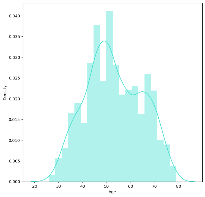
As we can see from the
groupbymethod, generation 4,5,and 6 contains a larger portion of customers. And later, I double check with the plot chart to see its indeed Customer’s age around 40-50 goes to the peak.
Customer’s income
Then, I want to see the relationship between customer’s income and the total amount of purchases they made.
Before that, I would like to narrow down the range of income, in case that the number is too large to considered as outliers.
df = df[df["Income"]<100000]
import altair as alt
brush = alt.selection_interval()
c1 = alt.Chart(df).mark_circle().encode(
    x=alt.X('Income', scale=alt.Scale(zero=False)),
    y='Total',
    color='Generation:N',
    tooltip=["ID", "Income", "Total"]
).add_selection(brush)

c2= alt.Chart(df).mark_bar().encode(
    x = 'ID',
    y='Total'
).transform_filter(brush)

c1|c2
Conclusion: We can see from this chart that there might be a positive relationship between the customers’ income and their total purchase. Later, I will use. regression to see if there’s a relation lie between them.
Linear and Polynomial Regression#
from sklearn.linear_model import LinearRegression
reg=LinearRegression()
reg.fit(df[["Income"]], df["Total"])
df["Pred"]=reg.predict(df[["Income"]])
df.head()
/shared-libs/python3.7/py-core/lib/python3.7/site-packages/ipykernel_launcher.py:4: SettingWithCopyWarning:
A value is trying to be set on a copy of a slice from a DataFrame.
Try using .loc[row_indexer,col_indexer] = value instead

See the caveats in the documentation: https://pandas.pydata.org/pandas-docs/stable/user_guide/indexing.html#returning-a-view-versus-a-copy
  after removing the cwd from sys.path.
| ID | Year_Birth | Education | Marital_Status | Income | Dt_Customer | Recency | Wines | Fruits | Meat | ... | AcceptedCmp4 | AcceptedCmp5 | AcceptedCmp1 | AcceptedCmp2 | Complain | Response | Total | Age | Generation | Pred | |
|---|---|---|---|---|---|---|---|---|---|---|---|---|---|---|---|---|---|---|---|---|---|
| 0 | 5524 | 1957 | Graduation | Single | 58138.0 | 04-09-2012 | 58 | 635 | 88 | 546 | ... | 0 | 0 | 0 | 0 | 0 | 1 | 1617 | 65 | 6 | 764.700135 |
| 1 | 2174 | 1954 | Graduation | Single | 46344.0 | 08-03-2014 | 38 | 11 | 1 | 6 | ... | 0 | 0 | 0 | 0 | 0 | 0 | 27 | 68 | 6 | 479.933385 |
| 2 | 4141 | 1965 | Graduation | Relationship | 71613.0 | 21-08-2013 | 26 | 426 | 49 | 127 | ... | 0 | 0 | 0 | 0 | 0 | 0 | 776 | 57 | 5 | 1090.054719 |
| 3 | 6182 | 1984 | Graduation | Relationship | 26646.0 | 10-02-2014 | 26 | 11 | 4 | 20 | ... | 0 | 0 | 0 | 0 | 0 | 0 | 53 | 38 | 3 | 4.324138 |
| 4 | 5324 | 1981 | PhD | Relationship | 58293.0 | 19-01-2014 | 94 | 173 | 43 | 118 | ... | 0 | 0 | 0 | 0 | 0 | 0 | 422 | 41 | 4 | 768.442619 |
5 rows × 29 columns
c = alt.Chart(df).mark_circle().encode(
    x=alt.X('Income', scale=alt.Scale(zero=False)),
    y=alt.Y('Total', scale=alt.Scale(zero=False)),
    color="ID"
)
c1=alt.Chart(df).mark_line(color="red").encode(
    x=alt.X('Income', scale=alt.Scale(zero=False)),
    y="Pred"
)
c+c1
By the graph above, we can easily confirm that there is a positive trend between customers’ income and total amount of purchase.
df["I2"]=df["Income"]**2
df["I3"]=df["Income"]**3
poly_cols = ["Income","I2", "I3"]
reg2 = LinearRegression()
reg2.fit(df[poly_cols], df["Total"])
df["poly_pred"] = reg2.predict(df[poly_cols])
/shared-libs/python3.7/py-core/lib/python3.7/site-packages/ipykernel_launcher.py:1: SettingWithCopyWarning:
A value is trying to be set on a copy of a slice from a DataFrame.
Try using .loc[row_indexer,col_indexer] = value instead

See the caveats in the documentation: https://pandas.pydata.org/pandas-docs/stable/user_guide/indexing.html#returning-a-view-versus-a-copy
  """Entry point for launching an IPython kernel.
/shared-libs/python3.7/py-core/lib/python3.7/site-packages/ipykernel_launcher.py:2: SettingWithCopyWarning:
A value is trying to be set on a copy of a slice from a DataFrame.
Try using .loc[row_indexer,col_indexer] = value instead

See the caveats in the documentation: https://pandas.pydata.org/pandas-docs/stable/user_guide/indexing.html#returning-a-view-versus-a-copy

/shared-libs/python3.7/py-core/lib/python3.7/site-packages/ipykernel_launcher.py:6: SettingWithCopyWarning:
A value is trying to be set on a copy of a slice from a DataFrame.
Try using .loc[row_indexer,col_indexer] = value instead

See the caveats in the documentation: https://pandas.pydata.org/pandas-docs/stable/user_guide/indexing.html#returning-a-view-versus-a-copy
c = alt.Chart(df).mark_circle().encode(
    x=alt.X('Income', scale=alt.Scale(zero=False)),
    y=alt.Y('Total', scale=alt.Scale(zero=False)),
    color="ID"
)

c1 = alt.Chart(df).mark_line(color="black").encode(
    x=alt.X('Income', scale=alt.Scale(zero=False)),
    y="poly_pred"
)

c+c1
Using polynomial regression to check, we can see the line it’s not strictly positive or negative, but its mostly positive.
Logistic Regression#
For this section, I want to add one feature in our analysis: “Marital_Status”. I am interested in predicting the customer’ marital status by their income and total amount spent on products.
from sklearn.linear_model import LogisticRegression #import
from sklearn.preprocessing import StandardScaler
from sklearn.model_selection import train_test_split
import numpy as np
# Make a sub-dataframe that only containes the necessary input that we want to predict
cols = ["Income","Total"]
df["Rel1"]=(df["Marital_Status"]== "Relationship") #Make the new colnmn that returns "True" if the customer is in a relationship, otherwise returns "False".
/shared-libs/python3.7/py-core/lib/python3.7/site-packages/ipykernel_launcher.py:3: SettingWithCopyWarning:
A value is trying to be set on a copy of a slice from a DataFrame.
Try using .loc[row_indexer,col_indexer] = value instead

See the caveats in the documentation: https://pandas.pydata.org/pandas-docs/stable/user_guide/indexing.html#returning-a-view-versus-a-copy
  This is separate from the ipykernel package so we can avoid doing imports until
Because our original dataset has a large sample size, making a train_test_split to divide dataset would make better and more accurate prediction.
X_train, X_test, y_train, y_test = train_test_split(df[cols], df["Rel1"], test_size=0.4, random_state=0)
clf=LogisticRegression()
clf.fit(X_train, y_train) #fit
(clf.predict(X_test) == y_test).sum() # Frequency
565
# The proportion that we made correct prediction based on the whole dataset.
(clf.predict(X_test) == y_test).sum()/len(X_test)
0.6355455568053994
The following step is to make sure that we get the right coefficient by specifing the index.
clf.coef_
Income_coef,Total_coef=clf.coef_[0]
Total_coef
-0.000449150869429734
From the coefficient that we get from the logistic prediction, we can tell that there is little relationship between the input:Income and Total with the output:Maritial_Status. Thus, it means it might not be higher income and more total will indicate if a customeris in a relationship.
Q:What will our model predict if we have the income for 71613 and the total amount is 776?
sigmoid = lambda x: 1/(1+np.exp(-x))
Income = 71613
Total = 776
sigmoid(Income_coef*Income+Total_coef*Total+clf.intercept_)
array([0.69477663])
Therefore,our model predicts that this customer with(income is $71613 and total is 776) has a 69.5% chance of being in a relationship.
Then we will double check with predict_proba.
clf.predict_proba([[Income,Total]])
/shared-libs/python3.7/py/lib/python3.7/site-packages/sklearn/base.py:451: UserWarning: X does not have valid feature names, but LogisticRegression was fitted with feature names
  "X does not have valid feature names, but"
array([[0.30522337, 0.69477663]])
The first array says that there is a 30.5% chance of this customer to be single(not in a relationship), and the second array gives the same result as the sigmoid function gives.
K-nearest Neighbor Classification#
#Import
from sklearn.neighbors import KNeighborsClassifier
from sklearn.metrics import log_loss
clf = KNeighborsClassifier()
clf.fit(X_train, y_train)
loss_train=log_loss(y_train, clf.predict_proba(X_train))
loss_test=log_loss(y_test,clf.predict_proba(X_test))
loss_train
0.5008396930029373
The log loss for x_train and y_train is about 0.501.
loss_test
2.4543962118660634
The log loss for x_test and y_test is about 2.454.
Therefore, we can see that loss_test is larger than loss_train, indicating a sign of over-fitting.
Decision Tree Classification#
Customer’s Eduction
Next, I will use Machine Learning: Decision Tree Classfier in order to use customer’s income, generation, and total amount of purchase to predict their education level.
# Import
from sklearn.tree import DecisionTreeClassifier
#Normalize the "Education" column
df["Education"]=df["Education"].replace({"Basic":"Undergraduate","2n Cycle":"Undergraduate", "Graduation":"Graduate", "Master":"Postgraduate", "PhD":"Postgraduate"})
/shared-libs/python3.7/py-core/lib/python3.7/site-packages/ipykernel_launcher.py:1: SettingWithCopyWarning:
A value is trying to be set on a copy of a slice from a DataFrame.
Try using .loc[row_indexer,col_indexer] = value instead

See the caveats in the documentation: https://pandas.pydata.org/pandas-docs/stable/user_guide/indexing.html#returning-a-view-versus-a-copy
  """Entry point for launching an IPython kernel.
input = ["Income","Total","Generation"]
X =df[input]
y = df["Education"]
X_train, X_test, y_train, y_test = train_test_split(X, y, train_size=0.6, random_state=49196138)
clf = DecisionTreeClassifier(max_leaf_nodes=8)
clf.fit(X_train, y_train) # Fit the classifier to the training data using X for the input features and using "Education" for the target.
DecisionTreeClassifier(max_leaf_nodes=8)
clf.score(X_train, y_train)
0.5476369092273068
clf.score(X_test, y_test)
0.4904386951631046
# Illustrate the resulting tree using matplotlib.
import matplotlib.pyplot as plt
from sklearn.tree import plot_tree
fig = plt.figure()
_ = plot_tree(clf,
                   feature_names=clf.feature_names_in_,
                   class_names=clf.classes_,
                   filled=True)
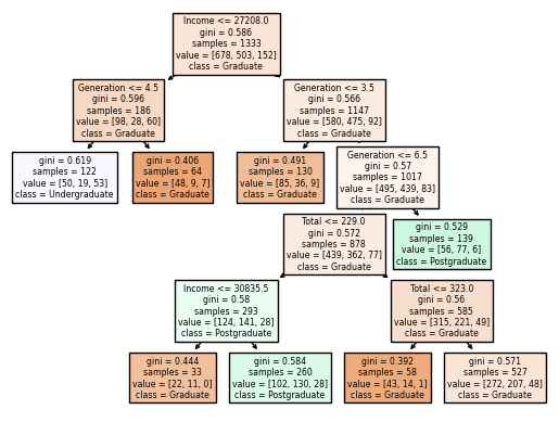
clf.feature_importances_
array([0.46173322, 0.17048733, 0.36777944])
pd.Series(clf.feature_importances_, index=clf.feature_names_in_)
Income        0.461733
Total         0.170487
Generation    0.367779
dtype: float64
Feature importance is a score assigned to the features of a Machine Learning model that defines how “important” is a feature to the model’s prediction. The feature_importance for Income, Total,and Generation are: 0.462, 0.170, and 0.368. Thus, we can know that “Income” is the most important feature to predict our model’s prediction.
Summary#
For this project, I first make a graph to show the distribution of the customer's generation. Then I used different regresion, including linear, polynomial, and logitic to show if there's relation between one's income and one's total amount of purchase. And the results showed that there's a position relationship between them. Later, I found out that Income is the the most significant feature to include when I want to predict our model's prediction for education.
References#
Your code above should include references. Here is some additional space for references.
What is the source of your dataset(s)?
Customer Personality Analysis: https://www.kaggle.com/datasets/imakash3011/customer-personality-analysis?datasetId=1546318&sortBy=voteCount.
List any other references that you found helpful.
Reference of code of logic regression: Course Notes from Spring 2022: https://christopherdavisuci.github.io/UCI-Math-10-S22/Week7/Week7-Friday.html . Reference of code of K-Nearest Neighbor regression: Course Notes from Winter 2022: https://christopherdavisuci.github.io/UCI-Math-10-W22/Week6/Week6-Wednesday.html . Reference for interactivity altair chart: https://altair-viz.github.io/altair-tutorial/notebooks/06-Selections.html. Reference for Decision Tree Classification and feature_importance: Week 8 Friday lecture: https://deepnote.com/workspace/math-10-f22-9ae9e411-d47b-4572-803e-16ff3e4d5a91/project/Week-8-Friday-12247a05-0b55-4f3c-b8d4-d2ccff50a983/notebook/Week8-Friday-59883ec6c3aa4332a20da4d2653f85e1.
Submission#
Using the Share button at the top right, enable Comment privileges for anyone with a link to the project. Then submit that link on Canvas.
 Created in Deepnote