Car Price Prediction#

Author: Kexin Sun

Course Project, UC Irvine, Math 10, F22

Introduction#

My project is to predict the price of future cars by analyzing the data in the data set. I first found out the brands with high sales volume, and then determined the factors affecting the price of the car by analyzing the correlation between various variables. I used Linear regression and train_test_split to analyze the prediction. I mainly analyzed the three most important factors: enginesize, curbweight, and horsepower to increase the accuracy of the model.

Main portion of the project#

Data Loading#

import pandas as pd
import altair as alt
import seaborn as sns
import matplotlib.pyplot as plt
import plotly.express as px
from sklearn.linear_model import LinearRegression
from sklearn.model_selection import train_test_split
from sklearn.preprocessing import StandardScaler
from sklearn.metrics import mean_squared_error
from sklearn.metrics import r2_score

df=pd.read_csv("CarPrice_Assignment.csv")
df

	car_ID	symboling	CarName	fueltype	aspiration	doornumber	carbody	drivewheel	enginelocation	wheelbase	...	enginesize	fuelsystem	boreratio	stroke	compressionratio	horsepower	peakrpm	citympg	highwaympg	price
0	1	3	alfa-romero giulia	gas	std	two	convertible	rwd	front	88.6	...	130	mpfi	3.47	2.68	9.0	111	5000	21	27	13495.0
1	2	3	alfa-romero stelvio	gas	std	two	convertible	rwd	front	88.6	...	130	mpfi	3.47	2.68	9.0	111	5000	21	27	16500.0
2	3	1	alfa-romero Quadrifoglio	gas	std	two	hatchback	rwd	front	94.5	...	152	mpfi	2.68	3.47	9.0	154	5000	19	26	16500.0
3	4	2	audi 100 ls	gas	std	four	sedan	fwd	front	99.8	...	109	mpfi	3.19	3.40	10.0	102	5500	24	30	13950.0
4	5	2	audi 100ls	gas	std	four	sedan	4wd	front	99.4	...	136	mpfi	3.19	3.40	8.0	115	5500	18	22	17450.0
...	...	...	...	...	...	...	...	...	...	...	...	...	...	...	...	...	...	...	...	...	...
200	201	-1	volvo 145e (sw)	gas	std	four	sedan	rwd	front	109.1	...	141	mpfi	3.78	3.15	9.5	114	5400	23	28	16845.0
201	202	-1	volvo 144ea	gas	turbo	four	sedan	rwd	front	109.1	...	141	mpfi	3.78	3.15	8.7	160	5300	19	25	19045.0
202	203	-1	volvo 244dl	gas	std	four	sedan	rwd	front	109.1	...	173	mpfi	3.58	2.87	8.8	134	5500	18	23	21485.0
203	204	-1	volvo 246	diesel	turbo	four	sedan	rwd	front	109.1	...	145	idi	3.01	3.40	23.0	106	4800	26	27	22470.0
204	205	-1	volvo 264gl	gas	turbo	four	sedan	rwd	front	109.1	...	141	mpfi	3.78	3.15	9.5	114	5400	19	25	22625.0

205 rows × 26 columns

df.shape

(205, 26)

df.isna().any().any()

False

df["Brand"]=df["CarName"].apply(lambda x:x.split(" ")[0])
df["Brand"].unique()

array(['alfa-romero', 'audi', 'bmw', 'chevrolet', 'dodge', 'honda',
       'isuzu', 'jaguar', 'maxda', 'mazda', 'buick', 'mercury',
       'mitsubishi', 'Nissan', 'nissan', 'peugeot', 'plymouth', 'porsche',
       'porcshce', 'renault', 'saab', 'subaru', 'toyota', 'toyouta',
       'vokswagen', 'volkswagen', 'vw', 'volvo'], dtype=object)

df=df.copy()

df=df.replace(['alfa-romero','maxda','Nissan','porschce','toyouta','vokswagen','volkswagen'],['alfa-romeo','mazda','nissan','porsche','toyota','vw','vw'])

df.drop("CarName",axis=1,inplace=True)

Data Visualization#

c = alt.Chart(df).mark_bar().encode(
    x = "Brand",
    y = "count()",
    color="Brand"
).properties(title="Sales of Each Brand"
)
c

According to the above chart, we can see that Toyota has the highest sales volume.

avg=df.groupby("Brand")["price"].mean()
avg

Brand
alfa-romeo    15498.333333
audi          17859.166714
bmw           26118.750000
buick         33647.000000
chevrolet      6007.000000
dodge          7875.444444
honda          8184.692308
isuzu          8916.500000
jaguar        34600.000000
mazda         10652.882353
mercury       16503.000000
mitsubishi     9239.769231
nissan        10415.666667
peugeot       15489.090909
plymouth       7963.428571
porcshce      32528.000000
porsche       31118.625000
renault        9595.000000
saab          15223.333333
subaru         8541.250000
toyota         9885.812500
volvo         18063.181818
vw            10077.500000
Name: price, dtype: float64

fig = px.bar(df, x=avg.index, y=avg)
fig.show()

According to the above chart, we can see that the average selling price of Buick and Jaguar are higher than that of other brands.

Find the correlation#

df.dtypes

car_ID                int64
symboling             int64
fueltype             object
aspiration           object
doornumber           object
carbody              object
drivewheel           object
enginelocation       object
wheelbase           float64
carlength           float64
carwidth            float64
carheight           float64
curbweight            int64
enginetype           object
cylindernumber       object
enginesize            int64
fuelsystem           object
boreratio           float64
stroke              float64
compressionratio    float64
horsepower            int64
peakrpm               int64
citympg               int64
highwaympg            int64
price               float64
Brand                object
dtype: object

num_col = df.select_dtypes(exclude=['object']).columns
num = df[num_col].drop(['car_ID'],axis=1)

cormatrix=num.corr()# find the correlationship among the dataset
cormatrix

	symboling	wheelbase	carlength	carwidth	carheight	curbweight	enginesize	boreratio	stroke	compressionratio	horsepower	peakrpm	citympg	highwaympg	price
symboling	1.000000	-0.531954	-0.357612	-0.232919	-0.541038	-0.227691	-0.105790	-0.130051	-0.008735	-0.178515	0.070873	0.273606	-0.035823	0.034606	-0.079978
wheelbase	-0.531954	1.000000	0.874587	0.795144	0.589435	0.776386	0.569329	0.488750	0.160959	0.249786	0.353294	-0.360469	-0.470414	-0.544082	0.577816
carlength	-0.357612	0.874587	1.000000	0.841118	0.491029	0.877728	0.683360	0.606454	0.129533	0.158414	0.552623	-0.287242	-0.670909	-0.704662	0.682920
carwidth	-0.232919	0.795144	0.841118	1.000000	0.279210	0.867032	0.735433	0.559150	0.182942	0.181129	0.640732	-0.220012	-0.642704	-0.677218	0.759325
carheight	-0.541038	0.589435	0.491029	0.279210	1.000000	0.295572	0.067149	0.171071	-0.055307	0.261214	-0.108802	-0.320411	-0.048640	-0.107358	0.119336
curbweight	-0.227691	0.776386	0.877728	0.867032	0.295572	1.000000	0.850594	0.648480	0.168790	0.151362	0.750739	-0.266243	-0.757414	-0.797465	0.835305
enginesize	-0.105790	0.569329	0.683360	0.735433	0.067149	0.850594	1.000000	0.583774	0.203129	0.028971	0.809769	-0.244660	-0.653658	-0.677470	0.874145
boreratio	-0.130051	0.488750	0.606454	0.559150	0.171071	0.648480	0.583774	1.000000	-0.055909	0.005197	0.573677	-0.254976	-0.584532	-0.587012	0.553173
stroke	-0.008735	0.160959	0.129533	0.182942	-0.055307	0.168790	0.203129	-0.055909	1.000000	0.186110	0.080940	-0.067964	-0.042145	-0.043931	0.079443
compressionratio	-0.178515	0.249786	0.158414	0.181129	0.261214	0.151362	0.028971	0.005197	0.186110	1.000000	-0.204326	-0.435741	0.324701	0.265201	0.067984
horsepower	0.070873	0.353294	0.552623	0.640732	-0.108802	0.750739	0.809769	0.573677	0.080940	-0.204326	1.000000	0.131073	-0.801456	-0.770544	0.808139
peakrpm	0.273606	-0.360469	-0.287242	-0.220012	-0.320411	-0.266243	-0.244660	-0.254976	-0.067964	-0.435741	0.131073	1.000000	-0.113544	-0.054275	-0.085267
citympg	-0.035823	-0.470414	-0.670909	-0.642704	-0.048640	-0.757414	-0.653658	-0.584532	-0.042145	0.324701	-0.801456	-0.113544	1.000000	0.971337	-0.685751
highwaympg	0.034606	-0.544082	-0.704662	-0.677218	-0.107358	-0.797465	-0.677470	-0.587012	-0.043931	0.265201	-0.770544	-0.054275	0.971337	1.000000	-0.697599
price	-0.079978	0.577816	0.682920	0.759325	0.119336	0.835305	0.874145	0.553173	0.079443	0.067984	0.808139	-0.085267	-0.685751	-0.697599	1.000000

plt.figure(figsize = (20,20))
sns.heatmap(cormatrix, annot=True)
plt.show()

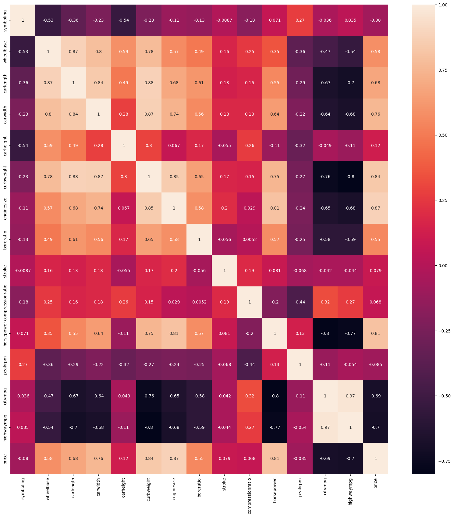
From this graph we can see the correlation between the two variables.

df["price"] = df["price"].astype(int)

df2 = df.copy()
df2 = df2.merge(avg.reset_index(),how="left",on= "Brand")
bins = [0,10000,20000,40000]
label = ["cheap","ordinary","expensive"]
df["price_level"] = pd.cut(df2["price_y"],bins,right=False,labels=label)
df

	car_ID	symboling	fueltype	aspiration	doornumber	carbody	drivewheel	enginelocation	wheelbase	carlength	...	boreratio	stroke	compressionratio	horsepower	peakrpm	citympg	highwaympg	price	Brand	price_level
0	1	3	gas	std	two	convertible	rwd	front	88.6	168.8	...	3.47	2.68	9.0	111	5000	21	27	13495	alfa-romeo	ordinary
1	2	3	gas	std	two	convertible	rwd	front	88.6	168.8	...	3.47	2.68	9.0	111	5000	21	27	16500	alfa-romeo	ordinary
2	3	1	gas	std	two	hatchback	rwd	front	94.5	171.2	...	2.68	3.47	9.0	154	5000	19	26	16500	alfa-romeo	ordinary
3	4	2	gas	std	four	sedan	fwd	front	99.8	176.6	...	3.19	3.40	10.0	102	5500	24	30	13950	audi	ordinary
4	5	2	gas	std	four	sedan	4wd	front	99.4	176.6	...	3.19	3.40	8.0	115	5500	18	22	17450	audi	ordinary
...	...	...	...	...	...	...	...	...	...	...	...	...	...	...	...	...	...	...	...	...	...
200	201	-1	gas	std	four	sedan	rwd	front	109.1	188.8	...	3.78	3.15	9.5	114	5400	23	28	16845	volvo	ordinary
201	202	-1	gas	turbo	four	sedan	rwd	front	109.1	188.8	...	3.78	3.15	8.7	160	5300	19	25	19045	volvo	ordinary
202	203	-1	gas	std	four	sedan	rwd	front	109.1	188.8	...	3.58	2.87	8.8	134	5500	18	23	21485	volvo	ordinary
203	204	-1	diesel	turbo	four	sedan	rwd	front	109.1	188.8	...	3.01	3.40	23.0	106	4800	26	27	22470	volvo	ordinary
204	205	-1	gas	turbo	four	sedan	rwd	front	109.1	188.8	...	3.78	3.15	9.5	114	5400	19	25	22625	volvo	ordinary

205 rows × 27 columns

The above are car brands in the same price range based on their average price.

cormatrix.sort_values(["price"], ascending = False, inplace = True)
print(cormatrix.price)

price               1.000000
enginesize          0.874145
curbweight          0.835305
horsepower          0.808139
carwidth            0.759325
carlength           0.682920
wheelbase           0.577816
boreratio           0.553173
carheight           0.119336
stroke              0.079443
compressionratio    0.067984
symboling          -0.079978
peakrpm            -0.085267
citympg            -0.685751
highwaympg         -0.697599
Name: price, dtype: float64

We find a strong positive correlation between enginesize, curbweight, horsepower, carwidth, carlength and car price, while a strong negative correlation between citympg, highwaympg and car price.（Positive correlation: When one variable increases, another will also increase; Negative correlation: An increase in one variable and a decrease in another.）

Create Linear Regression for the above 7 factors#

reg = LinearRegression()
cols=['curbweight','enginesize','horsepower','carwidth','carlength','citympg','highwaympg']
reg.fit(df[cols],df["price"])
pd.Series(reg.coef_,index=cols)

curbweight      3.083904
enginesize     83.155749
horsepower     47.807804
carwidth      630.832670
carlength     -31.697844
citympg       -61.820861
highwaympg     78.983351
dtype: float64

reg.intercept_

-47064.65162829726

reg.coef_

array([  3.08390409,  83.155749  ,  47.80780381, 630.83267019,
       -31.69784366, -61.82086051,  78.98335081])

df["Pred1"] = reg.predict(df[cols])
df

	car_ID	symboling	fueltype	aspiration	doornumber	carbody	drivewheel	enginelocation	wheelbase	carlength	...	stroke	compressionratio	horsepower	peakrpm	citympg	highwaympg	price	Brand	price_level	Pred1
0	1	3	gas	std	two	convertible	rwd	front	88.6	168.8	...	2.68	9.0	111	5000	21	27	13495	alfa-romeo	ordinary	12830.140148
1	2	3	gas	std	two	convertible	rwd	front	88.6	168.8	...	2.68	9.0	111	5000	21	27	16500	alfa-romeo	ordinary	12830.140148
2	3	1	gas	std	two	hatchback	rwd	front	94.5	171.2	...	3.47	9.0	154	5000	19	26	16500	alfa-romeo	ordinary	18415.125100
3	4	2	gas	std	four	sedan	fwd	front	99.8	176.6	...	3.40	10.0	102	5500	24	30	13950	audi	ordinary	11131.888319
4	5	2	gas	std	four	sedan	4wd	front	99.4	176.6	...	3.40	8.0	115	5500	18	22	17450	audi	ordinary	15365.681176
...	...	...	...	...	...	...	...	...	...	...	...	...	...	...	...	...	...	...	...	...	...
200	201	-1	gas	std	four	sedan	rwd	front	109.1	188.8	...	3.15	9.5	114	5400	23	28	16845	volvo	ordinary	17483.555626
201	202	-1	gas	turbo	four	sedan	rwd	front	109.1	188.8	...	3.15	8.7	160	5300	19	25	19045	volvo	ordinary	19929.103421
202	203	-1	gas	std	four	sedan	rwd	front	109.1	188.8	...	2.87	8.8	134	5500	18	23	21485	volvo	ordinary	21199.917464
203	204	-1	diesel	turbo	four	sedan	rwd	front	109.1	188.8	...	3.40	23.0	106	4800	26	27	22470	volvo	ordinary	17986.504844
204	205	-1	gas	turbo	four	sedan	rwd	front	109.1	188.8	...	3.15	9.5	114	5400	19	25	22625	volvo	ordinary	17833.118466

205 rows × 28 columns

We find seven factors that affect the price and make price forecast, which are enginesize, curbweight, horsepower, carwidth, carlength, citympg and highwaympg.

C=[]
for i in cols:
    c1=alt.Chart(df).mark_circle().encode(
        x=i,
        y="price",
        color="Brand"
    )
    C.append(c1)
alt.vconcat(*C)

The configuration of this Altair chart was adapted from https://christopherdavisuci.github.io/UCI-Math-10-S22/Proj/StudentProjects/KehanLi.html.

As can be seen from the figure above, enginesize, curbweight, horsepower, carwidth, carlength are positively correlated with price, while citympg, highwaympg are negatively correlated with price.

c2 = alt.Chart(df).mark_circle().encode(
    x="enginesize",
    y="price",
    color="Brand"
)
c3=alt.Chart(df).mark_line(color="Blue").encode(
    x="enginesize",
    y='Pred1',
)
c2+c3

Linear Regression for the most related 3 factor#

cols2=["enginesize","curbweight","horsepower"]

reg2=LinearRegression()
reg2.fit(df[cols2],df["price"])
df["Pred2"]=reg2.predict(df[cols2])

df

	car_ID	symboling	fueltype	aspiration	doornumber	carbody	drivewheel	enginelocation	wheelbase	carlength	...	compressionratio	horsepower	peakrpm	citympg	highwaympg	price	Brand	price_level	Pred1	Pred2
0	1	3	gas	std	two	convertible	rwd	front	88.6	168.8	...	9.0	111	5000	21	27	13495	alfa-romeo	ordinary	12830.140148	13842.478269
1	2	3	gas	std	two	convertible	rwd	front	88.6	168.8	...	9.0	111	5000	21	27	16500	alfa-romeo	ordinary	12830.140148	13842.478269
2	3	1	gas	std	two	hatchback	rwd	front	94.5	171.2	...	9.0	154	5000	19	26	16500	alfa-romeo	ordinary	18415.125100	18978.147751
3	4	2	gas	std	four	sedan	fwd	front	99.8	176.6	...	10.0	102	5500	24	30	13950	audi	ordinary	11131.888319	10721.878046
4	5	2	gas	std	four	sedan	4wd	front	99.4	176.6	...	8.0	115	5500	18	22	17450	audi	ordinary	15365.681176	15723.214753
...	...	...	...	...	...	...	...	...	...	...	...	...	...	...	...	...	...	...	...	...	...
200	201	-1	gas	std	four	sedan	rwd	front	109.1	188.8	...	9.5	114	5400	23	28	16845	volvo	ordinary	17483.555626	16644.477176
201	202	-1	gas	turbo	four	sedan	rwd	front	109.1	188.8	...	8.7	160	5300	19	25	19045	volvo	ordinary	19929.103421	19300.290806
202	203	-1	gas	std	four	sedan	rwd	front	109.1	188.8	...	8.8	134	5500	18	23	21485	volvo	ordinary	21199.917464	20591.319781
203	204	-1	diesel	turbo	four	sedan	rwd	front	109.1	188.8	...	23.0	106	4800	26	27	22470	volvo	ordinary	17986.504844	17723.606326
204	205	-1	gas	turbo	four	sedan	rwd	front	109.1	188.8	...	9.5	114	5400	19	25	22625	volvo	ordinary	17833.118466	17113.360474

205 rows × 29 columns

reg2.intercept_

-13463.82073148018

reg2.coef_

array([84.87987456,  4.26257543, 48.74660463])

std= StandardScaler()
std.fit(df[cols2])
X= std.transform(df[cols2])

y=df["price"]

X_train,X_test,y_train,y_test = train_test_split(X,y,test_size = 0.9, random_state=0)

X.shape

(205, 3)

M=LinearRegression()
M.fit(X_train,y_train)
M.score(X_train, y_train)

0.9087845055081182

M.score(X_test, y_test)

0.49538808151370906

print(f''' 
accuracy on Train score: {M.score(X_train, y_train):.1%}
accuracy on Test score: {M.score(X_test, y_test):.1%}
''')

 
accuracy on Train score: 90.9%
accuracy on Test score: 49.5%

pred=M.predict(X_test)

mean_squared_error(y_test, pred)

32337410.48764465

r2_score(y_test,pred)

0.49538808151370906

The model accounted for nearly 91% of the variance of the training data. But the score of testing data is too low, so it is not appropriate.

Summary#

I built a linear regression model to predict future car prices. After comparing the influence of various factors on the final result, I identified three key factors, namely enginesize, curbweight and horsepower. It is also found that citympg, highwaympg and price will be negatively correlated. Based on the analysis of the three main factors, the results show that the accuracy of the model is nearly 91% on the training data set and about 50% on the test data set. The R square of the model is about 50%.