Analyzing and Visualizing Top Soccer Data#

Author: Maria Avalos

Course Project, UC Irvine, Math 10, F22

Introduction#

Soccer has widely been known to be a global sport. Even those who are not familiar with it may recognize the names of some of the greates players, such as Lionel Messi or Javier “Chicharito” Hernandez. Anyone who is familiar with the sport may also recognize what the top teams are of their respective league, such as F.C. Barcelona for the spanish leage ‘La Liga’ or Manchester City for the English leage ‘the Premier League’. However what makes these teams to be able to constantly rank at the top? What could be the keys to their success. In this project, I explore data from the top European leagues to see what factors are affecting them the most to get theri high rankings using Regression models. I also explore where the top soccer teams are likely to score a goal to see get insight on success rates.

Importing and Cleaning the Data#

import pandas as pd
import altair as alt
import seaborn as sns
import matplotlib as mpl
import matplotlib.pyplot as plt
import random
from sklearn.model_selection import train_test_split
from pandas.api.types import is_numeric_dtype
from sklearn.tree import DecisionTreeRegressor
from sklearn.ensemble import RandomForestRegressor
from sklearn.metrics import mean_squared_error

df = pd.read_csv("EUClubSoccerStats.csv")
df

	Key	Team	League	Season	Rank	Games	Wins	Draws	Losses	Points	...	Nutmegs	Controlled	DistMovedWithBall	ProgressiveDistMoved	ProgC	ProgressiveIntoFinalThird	ProgressiveInto18Yard	Miscontrols	MiscontrolsAfterTackle	ProgressivePassReceived
0	Chelsea DL 2009/2010	Chelsea	Premier League	2009/2010	1.0	38.0	27.0	5.0	6.0	86.0	...	NaN	NaN	NaN	NaN	NaN	NaN	NaN	NaN	NaN	NaN
1	Manchester United DL 2009/2010	Manchester United	Premier League	2009/2010	2.0	38.0	27.0	4.0	7.0	85.0	...	NaN	NaN	NaN	NaN	NaN	NaN	NaN	NaN	NaN	NaN
2	Tottenham DL 2009/2010	Tottenham	Premier League	2009/2010	4.0	38.0	21.0	7.0	10.0	70.0	...	NaN	NaN	NaN	NaN	NaN	NaN	NaN	NaN	NaN	NaN
3	Arsenal DL 2009/2010	Arsenal	Premier League	2009/2010	3.0	38.0	23.0	6.0	9.0	75.0	...	NaN	NaN	NaN	NaN	NaN	NaN	NaN	NaN	NaN	NaN
4	Aston Villa DL 2009/2010	Aston Villa	Premier League	2009/2010	6.0	38.0	17.0	13.0	8.0	64.0	...	NaN	NaN	NaN	NaN	NaN	NaN	NaN	NaN	NaN	NaN
...	...	...	...	...	...	...	...	...	...	...	...	...	...	...	...	...	...	...	...	...	...
1685	Shakhtar Donetsk CL 2021/2022	Shakhtar Donetsk	Champions League	2021/2022	32.0	NaN	NaN	NaN	NaN	NaN	...	NaN	NaN	NaN	NaN	NaN	NaN	NaN	NaN	NaN	NaN
1686	FC Porto CL 2021/2022	FC Porto	Champions League	2021/2022	32.0	NaN	NaN	NaN	NaN	NaN	...	NaN	NaN	NaN	NaN	NaN	NaN	NaN	NaN	NaN	NaN
1687	Dynamo Kyiv CL 2021/2022	Dynamo Kyiv	Champions League	2021/2022	32.0	NaN	NaN	NaN	NaN	NaN	...	NaN	NaN	NaN	NaN	NaN	NaN	NaN	NaN	NaN	NaN
1688	Besiktas CL 2021/2022	Besiktas	Champions League	2021/2022	32.0	NaN	NaN	NaN	NaN	NaN	...	NaN	NaN	NaN	NaN	NaN	NaN	NaN	NaN	NaN	NaN
1689	Malmoe FF CL 2021/2022	Malmoe FF	Champions League	2021/2022	32.0	NaN	NaN	NaN	NaN	NaN	...	NaN	NaN	NaN	NaN	NaN	NaN	NaN	NaN	NaN	NaN

1690 rows × 93 columns

#checking if contains missing values
df.isnull().values.any()

True

Being that this is a pretty big DataFrame, it can be easy to miss but there are a good amount of missing values so we will clean it up. We will also drop the Key column as it won’t be needed.

df = df.dropna(axis=0).copy()
df = df.drop("Key", axis=1)
df.shape

(490, 92)

Since I want to investigate what factors effect a teams overall rank, I will first find the correlation among the dataset to the Rank and then create a sub-Dataframe containing those top factors as long as they are not repettive. Since Rank is from 1 being best to bigger number being worst, I have to check the ‘negative’ correlations as those will be the best. After finding it I will create my final Dataframe containing the averages stats of each team over the seasons to not overwhelm the data.

df.corr()["Rank"].sort_values(ascending=True).head(60)

Points                         -0.924545
Wins                           -0.915971
GoalDifference                 -0.913896
GoalsPerGame                   -0.812842
GoalsFor                       -0.804184
Goals                          -0.804063
TotalAssistPerGame             -0.784689
PenaltyAreaGoalsPerGame        -0.775376
OpenPlayGoals                  -0.773372
OtherAssistPerGame             -0.756561
ShotsOnTargetPer90             -0.722137
ShotsOnTarget                  -0.719465
LiveTouches                    -0.710984
Touches                        -0.708811
TotalPassesPerGame             -0.708256
TouchesAttPen                  -0.707056
ShortPassesPerGame             -0.703834
TouchesMidThird                -0.703194
AccShortPassesPerGame          -0.698008
TouchesAttThird                -0.697620
Controlled                     -0.696267
ProgC                          -0.695692
PenaltyAreaShotsPerGame        -0.688037
ShortKeyPassesPerGame          -0.685713
TotalKeyPassesPerGame          -0.683363
DistMovedWithBall              -0.673606
ProgressiveInto18Yard          -0.665003
ProgressiveDistMoved           -0.662875
TotalShotsPerGame              -0.660205
ProgressiveIntoFinalThird      -0.653073
PassSuccess                    -0.606517
ProgressivePassReceived        -0.598517
SixYardGoalsPerGame            -0.527219
Possession                     -0.511620
SixYardBoxShotsPerGame         -0.509078
ThroughballAssistPerGame       -0.503527
ThroughBallsPerGame            -0.498332
OutOfBoxGoalsPerGame           -0.488294
CounterAttackGoals             -0.431452
CrossAssistPerGame             -0.403930
SuccessfulDribblesPerGame      -0.400162
SetPieceGoals                  -0.392199
TotalDribblesPerGame           -0.378335
OutOfBoxShotsPerGame           -0.343887
NumOfPlayersDribbledPast       -0.333031
PenaltyGoals                   -0.321481
OwnGoals                       -0.303201
InAccurateShortPassesPerGame   -0.227660
OffsidesPerGame                -0.221775
UnsuccessfulDribblesPerGame    -0.202087
LongKeyPassesPerGame           -0.197566
Nutmegs                        -0.189896
AccurateLongBallsPerGame       -0.177729
TouchesDefThird                -0.172462
CornerAssistPerGame            -0.132320
CrossesPerGame                 -0.107073
FreekickAssistPerGame          -0.085647
MiscontrolsAfterTackle          0.006046
DisspossedPergame               0.015363
Games                           0.039848
Name: Rank, dtype: float64

df_sub = df.loc[:,['Team', 'League', 'Rank','Points', 'Wins', 'GoalDifference', 'GoalsPerGame','TotalAssistPerGame','OtherAssistPerGame', 'ShotsOnTargetPer90','Touches', 'TotalPassesPerGame','ShortPassesPerGame','TotalKeyPassesPerGame', 'DistMovedWithBall','TotalShotsPerGame','PassSuccess','Possession','SuccessfulDribblesPerGame']]
df_sub

	Team	League	Rank	Points	Wins	GoalDifference	GoalsPerGame	TotalAssistPerGame	OtherAssistPerGame	ShotsOnTargetPer90	Touches	TotalPassesPerGame	ShortPassesPerGame	TotalKeyPassesPerGame	DistMovedWithBall	TotalShotsPerGame	PassSuccess	Possession	SuccessfulDribblesPerGame
160	Manchester City	Premier League	1.0	100.0	32.0	79.0	2.8	2.2	1.4	6.710526	896.1	743.2	699	13.2	3119.5	17.5	89.0	66.4	13.2
161	Liverpool	Premier League	4.0	75.0	21.0	46.0	2.2	1.5	1.1	6.000000	768.5	604.3	546	12.9	2654.0	16.8	83.8	58.0	11.6
162	Manchester United	Premier League	2.0	81.0	25.0	40.0	1.8	1.4	0.9	4.631579	692.6	528.0	470	9.9	2285.4	13.5	83.6	53.9	12.3
163	Tottenham	Premier League	3.0	77.0	23.0	38.0	1.9	1.3	0.7	5.578947	743.9	570.0	509	12.3	2507.2	16.4	83.8	58.8	11.5
164	Chelsea	Premier League	5.0	70.0	21.0	24.0	1.6	1.1	0.6	5.500000	722.3	559.6	509	12.8	2534.3	15.9	84.3	54.4	13.5
...	...	...	...	...	...	...	...	...	...	...	...	...	...	...	...	...	...	...	...
1269	Bochum	Bundesliga	13.0	42.0	12.0	-14.0	1.2	0.7	0.4	4.117647	533.4	368.0	290	8.4	1600.8	12.1	72.1	44.5	6.8
1270	Augsburg	Bundesliga	14.0	38.0	10.0	-17.0	1.1	0.8	0.4	3.411765	507.6	336.5	274	7.7	1535.4	10.8	72.0	40.6	7.7
1271	Arminia Bielefeld	Bundesliga	17.0	28.0	5.0	-26.0	0.8	0.5	0.3	3.264706	521.2	356.8	294	7.3	1399.2	10.7	71.7	39.9	8.4
1272	Hertha Berlin	Bundesliga	16.0	33.0	9.0	-34.0	1.1	0.7	0.4	3.500000	541.1	370.0	317	8.0	1526.9	10.8	74.7	43.2	8.3
1273	Greuther Fuerth	Bundesliga	18.0	18.0	3.0	-54.0	0.8	0.4	0.2	2.764706	536.2	368.9	313	6.1	1563.6	9.2	74.8	43.0	7.8

490 rows × 19 columns

#taking average stats of every team for further analysis
df_avg = df_sub.groupby(["Team",'League'], sort=False, as_index=False).mean()
df_avg

	Team	League	Rank	Points	Wins	GoalDifference	GoalsPerGame	TotalAssistPerGame	OtherAssistPerGame	ShotsOnTargetPer90	Touches	TotalPassesPerGame	ShortPassesPerGame	TotalKeyPassesPerGame	DistMovedWithBall	TotalShotsPerGame	PassSuccess	Possession	SuccessfulDribblesPerGame
0	Manchester City	Premier League	1.200000	91.600000	29.200000	68.400000	2.56	1.800000	1.180000	6.326316	839.060000	699.600000	655.200000	13.680000	3135.80	17.940000	89.280000	64.40	12.300000
1	Liverpool	Premier League	2.400000	86.400000	26.200000	51.800000	2.20	1.540000	0.980000	5.784211	775.880000	622.900000	568.000000	12.420000	2531.54	16.540000	84.620000	59.70	10.180000
2	Manchester United	Premier League	3.800000	69.000000	19.800000	22.000000	1.72	1.220000	0.800000	5.068421	673.700000	522.900000	473.400000	10.440000	2309.72	13.760000	83.420000	53.68	10.600000
3	Tottenham	Premier League	4.800000	68.000000	20.400000	26.400000	1.78	1.220000	0.780000	4.757895	678.520000	525.420000	473.600000	9.960000	2216.80	13.360000	83.040000	54.04	10.700000
4	Chelsea	Premier League	3.800000	69.800000	20.400000	25.600000	1.72	1.220000	0.700000	5.273684	767.220000	614.900000	567.600000	12.280000	2666.84	15.700000	86.240000	58.60	11.280000
...	...	...	...	...	...	...	...	...	...	...	...	...	...	...	...	...	...	...	...
130	Union Berlin	Bundesliga	7.666667	49.333333	13.333333	-1.333333	1.40	0.966667	0.533333	4.078431	550.766667	388.566667	324.666667	8.566667	1621.00	11.866667	73.433333	36.00	6.966667
131	Paderborn	Bundesliga	18.000000	20.000000	4.000000	-37.000000	1.10	0.800000	0.500000	3.823529	577.000000	394.900000	344.000000	9.000000	2019.20	12.700000	77.800000	46.90	11.200000
132	Arminia Bielefeld	Bundesliga	16.000000	31.500000	7.000000	-26.000000	0.80	0.500000	0.300000	3.102941	533.100000	373.250000	307.500000	7.050000	1469.15	10.250000	73.150000	42.00	7.650000
133	Bochum	Bundesliga	13.000000	42.000000	12.000000	-14.000000	1.20	0.700000	0.400000	4.117647	533.400000	368.000000	290.000000	8.400000	1600.80	12.100000	72.100000	44.50	6.800000
134	Greuther Fuerth	Bundesliga	18.000000	18.000000	3.000000	-54.000000	0.80	0.400000	0.200000	2.764706	536.200000	368.900000	313.000000	6.100000	1563.60	9.200000	74.800000	43.00	7.800000

135 rows × 19 columns

#example visualization with one of those top factors
alt.Chart(df_avg).mark_circle().encode(
    x= alt.X('Rank', scale=alt.Scale(domain=(1,21),reverse=True)),
    y='Wins',
    color="League:N",
    tooltip = ["Team", 'Rank','League']
)

Predicting Factor Importance to Team Ranking#

Since I want to explore what factors are most important to a team to achieve higher ranking, in other words what factors make the top teams stay at the top,I decided to use regression to be able to find associations between these two things.

Decision Tree Regression#

#getting the features we are going to use for predicition
features = [col for col in df_avg.columns if is_numeric_dtype(df_avg[col]) & (col!='Rank') & (col!='Team')& (col!='League')& (col!='Season')]
features

['Points',
 'Wins',
 'GoalDifference',
 'GoalsPerGame',
 'TotalAssistPerGame',
 'OtherAssistPerGame',
 'ShotsOnTargetPer90',
 'Touches',
 'TotalPassesPerGame',
 'ShortPassesPerGame',
 'TotalKeyPassesPerGame',
 'DistMovedWithBall',
 'TotalShotsPerGame',
 'PassSuccess',
 'Possession',
 'SuccessfulDribblesPerGame']

X_train, X_test, y_train, y_test = train_test_split(df_avg[features], df_avg["Rank"], test_size=0.6, random_state=2868)

As we are aware that decision trees can denote problems such as overfitting or underfitting,we can create a u-shaped error model to find the best number of leaf nodes. This configuration was adapted a previous student and this site.

train_error_dict = {}
test_error_dict = {}
for n in range(2,80):
    reg = DecisionTreeRegressor(max_leaf_nodes=n,random_state=2868)
    reg.fit(X_train, y_train)
    train_error_dict[n]= mean_squared_error(y_train, reg.predict(X_train))
    test_error_dict[n]= mean_squared_error(y_test, reg.predict(X_test))

df_train = pd.DataFrame({"y":train_error_dict, "type": "train"})
df_test = pd.DataFrame({"y":test_error_dict, "type": "test"})
df_error = pd.concat([df_train, df_test]).reset_index()

alt.Chart(df_error).mark_line(clip=True).encode(
    x="index:O",
    y="y",
    color="type"
)

As we can see, n=6,7,8 are roughly where the best model is. Let’s use this and hope our numbers look nice.

reg = DecisionTreeRegressor(max_leaf_nodes=6)

reg.fit(X_train, y_train)

DecisionTreeRegressor(max_leaf_nodes=6)

reg.score(X_train, y_train)

0.953148281700124

reg.score(X_test, y_test)

0.8893122172264274

pd.Series(reg.feature_importances_, index=features).sort_values(ascending=False)

Wins                         0.854781
GoalDifference               0.128957
Points                       0.016262
GoalsPerGame                 0.000000
TotalAssistPerGame           0.000000
OtherAssistPerGame           0.000000
ShotsOnTargetPer90           0.000000
Touches                      0.000000
TotalPassesPerGame           0.000000
ShortPassesPerGame           0.000000
TotalKeyPassesPerGame        0.000000
DistMovedWithBall            0.000000
TotalShotsPerGame            0.000000
PassSuccess                  0.000000
Possession                   0.000000
SuccessfulDribblesPerGame    0.000000
dtype: float64

Lots of zero values.

df_importance = pd.DataFrame({"Importance": reg.feature_importances_, "Feature": reg.feature_names_in_})

alt.Chart(df_importance).mark_bar().encode(
    x="Importance",
    y="Feature",
    tooltip=["Importance", "Feature"],
).properties(
    title="Importance of factors affecting Team Rankings",
    width = 900
)

As we can see, this is not really that intersting. Of course realistically, it does make sense that the more Wins ones has, the higher their ranking. Let’s try for bigger nodes to see if we get more intersting results just for fun.

reg_fun = DecisionTreeRegressor(max_leaf_nodes=80)

reg_fun.fit(X_train, y_train)

DecisionTreeRegressor(max_leaf_nodes=80)

reg_fun.score(X_train, y_train)

1.0

reg_fun.score(X_test, y_test)

0.8493453236070818

pd.Series(reg_fun.feature_importances_, index=features).sort_values(ascending=False)

Wins                         0.772807
GoalDifference               0.125750
TotalShotsPerGame            0.048440
GoalsPerGame                 0.019328
Points                       0.015886
ShotsOnTargetPer90           0.005787
TotalAssistPerGame           0.002781
ShortPassesPerGame           0.002617
Possession                   0.002148
TotalPassesPerGame           0.001828
PassSuccess                  0.001123
SuccessfulDribblesPerGame    0.000797
Touches                      0.000498
DistMovedWithBall            0.000180
OtherAssistPerGame           0.000030
TotalKeyPassesPerGame        0.000000
dtype: float64

df_importance = pd.DataFrame({"Importance": reg_fun.feature_importances_, "Feature": reg_fun.feature_names_in_})

d_tree = alt.Chart(df_importance).mark_bar().encode(
    x="Importance",
    y="Feature",
    tooltip=["Importance", "Feature"],
).properties(
    title="Importance of factors affecting Team Ranking Using DecisionTree",
    width = 900
)
d_tree

Random Forest Regression#

Random Forest regression can sometimes help with the problem of overfitting since they combine the output of multiple decision trees to come up with the final prediciton. So I’ve decided to test it out and see if I’d be given a different result. Let’s check our error curve first.

train_error_dict = {}
test_error_dict = {}
for n in range(2,25):
    rfe = RandomForestRegressor(n_estimators=1000,max_leaf_nodes=n,random_state=2868)
    rfe.fit(X_train, y_train)
    train_error_dict[n]= mean_squared_error(y_train, rfe.predict(X_train))
    test_error_dict[n]= mean_squared_error(y_test, rfe.predict(X_test))

df_train = pd.DataFrame({"y":train_error_dict, "type": "train"})
df_test = pd.DataFrame({"y":test_error_dict, "type": "test"})
df_error = pd.concat([df_train, df_test]).reset_index()

alt.Chart(df_error).mark_line(clip=True).encode(
    x="index:O",
    y="y",
    color="type"
)

As we can see, we really only need n to be about 4 or 5 so we will have that in our first run.

rfe = RandomForestRegressor(n_estimators=1000, max_leaf_nodes=5,random_state=2868)

rfe.fit(X_train,y_train)

RandomForestRegressor(max_leaf_nodes=5, n_estimators=1000, random_state=2868)

rfe.score(X_train,y_train)

0.9631823907907027

rfe.score(X_test,y_test)

0.905822639881225

df_importance1 = pd.DataFrame({"importance": rfe.feature_importances_, "feature": rfe.feature_names_in_})

pd.Series(rfe.feature_importances_, index=features).sort_values(ascending=False)

Wins                         0.406344
Points                       0.261425
GoalDifference               0.162745
GoalsPerGame                 0.039579
TotalPassesPerGame           0.026745
TotalAssistPerGame           0.020673
Touches                      0.018476
ShortPassesPerGame           0.017766
PassSuccess                  0.011185
OtherAssistPerGame           0.006909
Possession                   0.006747
DistMovedWithBall            0.005791
TotalShotsPerGame            0.005604
TotalKeyPassesPerGame        0.005341
ShotsOnTargetPer90           0.004300
SuccessfulDribblesPerGame    0.000371
dtype: float64

We can already see better number results (no zero values).

rand_for = alt.Chart(df_importance1).mark_bar().encode(
    x="importance",
    y="feature",
    tooltip=["importance", "feature"],
).properties(
    title="Importance of factors affecting Blue's win using RandomForest",
    width = 900
)
rand_for

#comparison between the twoo
d_tree|rand_for

Overall, it is safe to conclude that based on the feature importances that I did to the data, Wins clearly are what affect a team’s ranking the most followed by Points and GoalDifference.

Visualizing Top Team Insights#

As we saw from my results, it appears that the amount of Wins a team gets, on average, throughout their season. But since soccer is a overall sport where one thing is affected by another (ex:rank is affected by wins which is affected by goals scored), I wanted to analyze where the Top Teams of two different leagues are more likely to score in hopes of demonstrating where one should attempt to score to get more points or getting some type of insight on their key to success.

Shot Map#

Here I will create two DataFrames containing the top 10 teams from La Liga, the Spanish league, and the Premier League, the English league.

liga = df[(df['League'] == 'La Liga') & (df['Rank']<= 10)]
liga = liga.loc[:,['Team','Rank','SixYardGoalsPerGame','PenaltyAreaGoalsPerGame','OutOfBoxGoalsPerGame']]
liga

	Team	Rank	SixYardGoalsPerGame	PenaltyAreaGoalsPerGame	OutOfBoxGoalsPerGame
420	Barcelona	1.0	0.6	1.6	0.3
421	Real Madrid	3.0	0.4	1.7	0.3
422	Atletico Madrid	2.0	0.2	1.1	0.2
423	Valencia	4.0	0.4	1.0	0.3
424	Villarreal	5.0	0.3	1.0	0.2
426	Sevilla	7.0	0.2	0.9	0.2
428	Real Betis	6.0	0.3	0.9	0.2
430	Girona	10.0	0.3	0.9	0.1
432	Eibar	9.0	0.3	0.7	0.2
434	Getafe	8.0	0.2	0.6	0.3
440	Barcelona	1.0	0.3	1.6	0.3
441	Atletico Madrid	2.0	0.4	0.7	0.4
442	Real Madrid	3.0	0.2	1.3	0.1
443	Valencia	4.0	0.3	0.9	0.1
444	Sevilla	6.0	0.4	1.1	0.1
447	Real Sociedad	9.0	0.2	0.9	0.1
448	Getafe	5.0	0.2	0.8	0.2
449	Espanyol	7.0	0.2	0.6	0.3
451	Real Betis	10.0	0.2	0.8	0.2
452	Athletic Bilbao	8.0	0.3	0.7	0.1
460	Real Madrid	1.0	0.3	1.4	0.2
461	Barcelona	2.0	0.2	1.6	0.4
462	Sevilla	4.0	0.3	0.9	0.2
463	Atletico Madrid	3.0	0.3	0.9	0.1
464	Villarreal	5.0	0.3	1.2	0.2
465	Real Sociedad	6.0	0.2	1.1	0.1
467	Granada	7.0	0.3	0.8	0.2
468	Osasuna	10.0	0.2	0.8	0.2
471	Getafe	8.0	0.3	0.8	0.1
472	Valencia	9.0	0.3	0.8	0.2
480	Barcelona	3.0	0.4	1.4	0.3
481	Real Madrid	2.0	0.4	1.1	0.2
482	Atletico Madrid	1.0	0.2	1.3	0.2
483	Sevilla	4.0	0.2	0.9	0.2
484	Villarreal	7.0	0.2	1.1	0.2
485	Real Sociedad	5.0	0.4	0.9	0.2
486	Real Betis	6.0	0.3	0.9	0.2
488	Celta Vigo	8.0	0.4	0.9	0.2
491	Athletic Bilbao	10.0	0.4	0.7	0.1
498	Granada	9.0	0.1	0.9	0.2
500	Real Madrid	1.0	0.6	1.4	0.2
501	Barcelona	2.0	0.4	1.2	0.2
502	Real Betis	5.0	0.3	1.0	0.3
503	Villarreal	7.0	0.5	1.1	0.1
504	Atletico Madrid	3.0	0.4	1.0	0.2
505	Sevilla	4.0	0.3	0.8	0.2
506	Real Sociedad	6.0	0.2	0.8	0.1
508	Athletic Bilbao	8.0	0.2	0.7	0.1
511	Osasuna	10.0	0.1	0.7	0.2
512	Valencia	9.0	0.2	0.9	0.1

premier = df[(df['League'] == 'Premier League') & (df['Rank']<= 10)]
premier = premier.loc[:,['Team','Rank','SixYardGoalsPerGame','PenaltyAreaGoalsPerGame','OutOfBoxGoalsPerGame']]
premier

	Team	Rank	SixYardGoalsPerGame	PenaltyAreaGoalsPerGame	OutOfBoxGoalsPerGame
160	Manchester City	1.0	0.7	1.7	0.3
161	Liverpool	4.0	0.4	1.5	0.2
162	Manchester United	2.0	0.3	1.1	0.3
163	Tottenham	3.0	0.4	1.2	0.3
164	Chelsea	5.0	0.3	1.0	0.3
165	Arsenal	6.0	0.4	1.4	0.2
167	Burnley	7.0	0.2	0.6	0.1
168	Leicester	9.0	0.4	0.8	0.2
170	Newcastle	10.0	0.3	0.6	0.1
173	Everton	8.0	0.2	0.7	0.2
180	Manchester City	1.0	0.5	1.5	0.4
181	Liverpool	2.0	0.5	1.6	0.1
182	Chelsea	3.0	0.2	1.2	0.2
183	Tottenham	4.0	0.4	0.9	0.4
184	Arsenal	5.0	0.4	1.2	0.3
186	Leicester	9.0	0.2	0.8	0.2
187	West Ham	10.0	0.4	0.8	0.1
188	Everton	8.0	0.3	0.9	0.2
189	Wolverhampton	7.0	0.3	0.9	0.1
190	Manchester United	6.0	0.4	1.1	0.3
200	Manchester City	2.0	0.6	1.6	0.4
201	Liverpool	1.0	0.3	1.6	0.3
202	Leicester	5.0	0.4	1.1	0.2
203	Chelsea	4.0	0.3	1.2	0.3
204	Manchester United	3.0	0.2	1.2	0.3
205	Wolverhampton	7.0	0.4	0.7	0.2
206	Tottenham	6.0	0.3	1.0	0.2
207	Burnley	10.0	0.3	0.6	0.2
208	Sheffield United	9.0	0.2	0.7	0.0
210	Arsenal	8.0	0.3	1.0	0.1
220	Manchester City	1.0	0.4	1.5	0.3
221	Manchester United	2.0	0.2	1.4	0.2
223	Chelsea	4.0	0.3	1.1	0.1
224	Liverpool	3.0	0.3	1.3	0.2
225	Tottenham	7.0	0.4	1.0	0.3
226	Leicester	5.0	0.2	1.2	0.3
227	Leeds	9.0	0.3	0.9	0.3
228	West Ham	6.0	0.6	0.9	0.1
229	Everton	10.0	0.5	0.6	0.1
230	Arsenal	8.0	0.3	1.0	0.1
240	Manchester City	1.0	0.7	1.4	0.4
241	Liverpool	2.0	0.7	1.6	0.2
242	Chelsea	3.0	0.4	1.3	0.3
243	Tottenham	4.0	0.3	1.1	0.2
244	West Ham	7.0	0.4	0.9	0.2
245	Manchester United	6.0	0.2	1.1	0.2
247	Arsenal	5.0	0.4	0.9	0.3
248	Leicester	8.0	0.2	1.2	0.2
249	Brighton	9.0	0.2	0.7	0.2
250	Wolverhampton	10.0	0.2	0.6	0.2

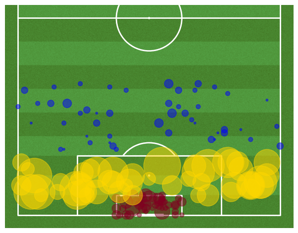
Unfortunately, this data did not come with the coordinates to plot where these shots were taken for our shot map we will have to create our own. Luckily, there are statistics on where on the field the team averaged to score per game so we can create a rough estimate.

#points for 'La Liga' teams
y_s = [random.randint(114,120) for i in range(50)]
liga['y_s'] = y_s
x_s= [random.randint(30,50) for i in range(50)]
liga['x_s'] = x_s
y_p = [random.randint(104,114) for i in range(50)]
liga['y_p'] = y_p
x_p = [random.randint(0,80) for i in range(50)]
liga['x_p'] = x_p
y_o = [random.randint(80,100) for i in range(50)]
liga['y_o'] = y_o
x_o = [random.randint(0,80) for i in range(50)]
liga['x_o'] = x_o

#points for 'Premier League' Teams
y_s = [random.randint(114,120) for i in range(50)]
premier['y_s'] = y_s
x_s= [random.randint(30,50) for i in range(50)]
premier['x_s'] = x_s
y_p = [random.randint(104,114) for i in range(50)]
premier['y_p'] = y_p
x_p = [random.randint(0,80) for i in range(50)]
premier['x_p'] = x_p
y_o = [random.randint(80,100) for i in range(50)]
premier['y_o'] = y_o
x_o = [random.randint(0,80) for i in range(50)]
premier['x_o'] = x_o

#size of points to be the amount of times they scored
size_s = liga['SixYardGoalsPerGame'].to_numpy()
s_s = [1000*s_s**2 for s_s in size_s]
size_p = liga['PenaltyAreaGoalsPerGame'].to_numpy()
s_p = [1000*s_p**2 for s_p in size_p]
size_o = liga['OutOfBoxGoalsPerGame'].to_numpy()
s_o = [1000*s_o**2 for s_o in size_o]

size_s = premier['SixYardGoalsPerGame'].to_numpy()
s_s = [1000*s_s**2 for s_s in size_s]
size_p = premier['PenaltyAreaGoalsPerGame'].to_numpy()
s_p = [1000*s_p**2 for s_p in size_p]
size_o = premier['OutOfBoxGoalsPerGame'].to_numpy()
s_o = [1000*s_o**2 for s_o in size_o]

Looking at analysis that have been done with soccer statistics I found this website that has a program that assists with creating visualizations so that is what I will use.

#install the program for graphics
!pip install mplsoccer==1.1.9

Requirement already satisfied: mplsoccer==1.1.9 in /root/venv/lib/python3.7/site-packages (1.1.9)
Requirement already satisfied: matplotlib in /shared-libs/python3.7/py/lib/python3.7/site-packages (from mplsoccer==1.1.9) (3.5.3)
Requirement already satisfied: scipy in /shared-libs/python3.7/py/lib/python3.7/site-packages (from mplsoccer==1.1.9) (1.7.3)
Requirement already satisfied: pillow in /shared-libs/python3.7/py/lib/python3.7/site-packages (from mplsoccer==1.1.9) (9.2.0)
Requirement already satisfied: seaborn in /shared-libs/python3.7/py/lib/python3.7/site-packages (from mplsoccer==1.1.9) (0.12.1)
Requirement already satisfied: requests in /shared-libs/python3.7/py/lib/python3.7/site-packages (from mplsoccer==1.1.9) (2.28.1)
Requirement already satisfied: pandas in /shared-libs/python3.7/py/lib/python3.7/site-packages (from mplsoccer==1.1.9) (1.2.5)
Requirement already satisfied: numpy in /shared-libs/python3.7/py/lib/python3.7/site-packages (from mplsoccer==1.1.9) (1.21.6)
Requirement already satisfied: pyparsing>=2.2.1 in /shared-libs/python3.7/py-core/lib/python3.7/site-packages (from matplotlib->mplsoccer==1.1.9) (3.0.9)
Requirement already satisfied: kiwisolver>=1.0.1 in /shared-libs/python3.7/py/lib/python3.7/site-packages (from matplotlib->mplsoccer==1.1.9) (1.4.4)
Requirement already satisfied: fonttools>=4.22.0 in /shared-libs/python3.7/py/lib/python3.7/site-packages (from matplotlib->mplsoccer==1.1.9) (4.37.4)
Requirement already satisfied: cycler>=0.10 in /shared-libs/python3.7/py/lib/python3.7/site-packages (from matplotlib->mplsoccer==1.1.9) (0.11.0)
Requirement already satisfied: python-dateutil>=2.7 in /shared-libs/python3.7/py-core/lib/python3.7/site-packages (from matplotlib->mplsoccer==1.1.9) (2.8.2)
Requirement already satisfied: packaging>=20.0 in /shared-libs/python3.7/py-core/lib/python3.7/site-packages (from matplotlib->mplsoccer==1.1.9) (21.3)
Requirement already satisfied: pytz>=2017.3 in /shared-libs/python3.7/py/lib/python3.7/site-packages (from pandas->mplsoccer==1.1.9) (2022.5)
Requirement already satisfied: certifi>=2017.4.17 in /shared-libs/python3.7/py/lib/python3.7/site-packages (from requests->mplsoccer==1.1.9) (2022.9.24)
Requirement already satisfied: idna<4,>=2.5 in /shared-libs/python3.7/py-core/lib/python3.7/site-packages (from requests->mplsoccer==1.1.9) (3.4)
Requirement already satisfied: charset-normalizer<3,>=2 in /shared-libs/python3.7/py-core/lib/python3.7/site-packages (from requests->mplsoccer==1.1.9) (2.1.1)
Requirement already satisfied: urllib3<1.27,>=1.21.1 in /shared-libs/python3.7/py/lib/python3.7/site-packages (from requests->mplsoccer==1.1.9) (1.26.12)
Requirement already satisfied: typing_extensions in /shared-libs/python3.7/py-core/lib/python3.7/site-packages (from seaborn->mplsoccer==1.1.9) (4.4.0)
Requirement already satisfied: six>=1.5 in /shared-libs/python3.7/py-core/lib/python3.7/site-packages (from python-dateutil>=2.7->matplotlib->mplsoccer==1.1.9) (1.16.0)
WARNING: You are using pip version 22.0.4; however, version 22.3.1 is available.
You should consider upgrading via the '/root/venv/bin/python -m pip install --upgrade pip' command.

from mplsoccer.pitch import VerticalPitch

pitch = VerticalPitch(half=True,pitch_color='grass', line_color='white', stripe=True)
fig, ax = pitch.draw()
plt.gca().invert_yaxis()
#scatter plot of goal locations
plt.scatter(liga['x_s'],liga['y_s'],s=s_s, c = "#800020",alpha=0.5)
plt.scatter(liga['x_p'],liga['y_p'],s=s_p, c = "#FFD700",alpha=0.5)
plt.scatter(liga['x_o'],liga['y_o'],s=s_o, c = "#0000FF",alpha=0.5)

<matplotlib.collections.PathCollection at 0x7fcf7cafc110>

pitch = VerticalPitch(half=True,pitch_color='grass', line_color='white', stripe=True)
fig, ax = pitch.draw()
plt.gca().invert_yaxis()
#scatter plot of goal locations
plt.scatter(premier['x_s'],premier['y_s'],s=s_s, c = "#800020",alpha=0.5)
plt.scatter(premier['x_p'],premier['y_p'],s=s_p, c = "#FFD700",alpha=0.5)
plt.scatter(premier['x_o'],premier['y_o'],s=s_o, c = "#0000FF",alpha=0.5)

<matplotlib.collections.PathCollection at 0x7fcf7c9bee50>

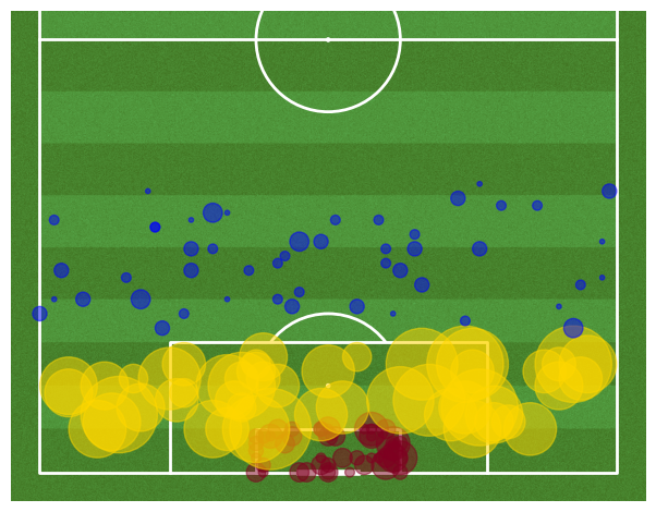
Both top teams from both leagues seem to have the most success making a goal if they shoot anywhere in the penalty area distance as this is wheere the points are the biggest.

Heat Map#

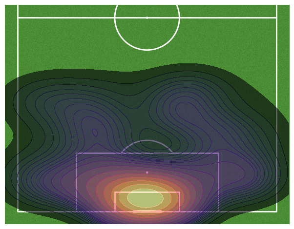
Another visualization that can help us is a heat map to see where the most activity is happening. Let’s try.

#getting the goal point locations only
x_points = liga.melt(value_vars = ['x_s','x_p','x_o'])
y_points = liga.melt(value_vars = ['y_s','y_p','y_o'])
liga_pts = pd.DataFrame({'x_points':x_points['value'],'y_points':y_points['value']})

x_points = premier.melt(value_vars = ['x_s','x_p','x_o'])
y_points = premier.melt(value_vars = ['y_s','y_p','y_o'])
premier_pts = pd.DataFrame({'x_points':x_points['value'],'y_points':y_points['value']})

pitch = VerticalPitch(half=True,pitch_color='grass', line_color='white')
fig, ax = pitch.draw()
plt.gca().invert_yaxis()
#heat map
kde1 = sns.kdeplot(
    x = liga_pts['x_points'],
    y = liga_pts['y_points'],
    levels=20,
    fill=True,
    alpha=0.6,
    cmap = 'magma'
)
kde1

<AxesSubplot:xlabel='x_points', ylabel='y_points'>

pitch = VerticalPitch(half=True,pitch_color='grass', line_color='white')
fig, ax = pitch.draw()
plt.gca().invert_yaxis()
#heat map
kde2 = sns.kdeplot(
    x = premier_pts['x_points'],
    y = premier_pts['y_points'],
    levels=20,
    fill=True,
    alpha=0.6,
    cmap = 'magma'
)

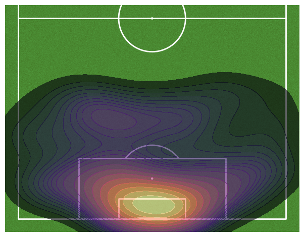
Proving our initial scatter plot conclusion, here we can see that indeed, most of the activity when scoring goals happens Six Yards from the goal post and the Penalty Area.

Summary#

After testing using two different models, DecisionTree Regression and RandomForest Regression, I was able to get an insight on what are the most important factors that affect a teams rankings. Clearly the top teams are the top teams because they Win and Score the most. Goal difference is also important, which makes sense as scoring the most is not important if you are getting scored on just as much, cancelling out any progress. I was also able to conclude, from my visualizations, that the tops teams score the most when they shoot in the 6-yard area the most followed by the penalty area.

References#

Your code above should include references. Here is some additional space for references.

What is the source of your dataset(s)?

Source : Performance Data on Football teams 09 to 22

List any other references that you found helpful.

Submission#

Using the Share button at the top right, enable Comment privileges for anyone with a link to the project. Then submit that link on Canvas.

Created in Deepnote

UC Irvine Math 10, Fall 2022

Analyzing and Visualizing Top Soccer Data

Contents