Salary Classification By Using Decision Tree#

Author: Kevin Xu

Course Project, UC Irvine, Math 10, F22

Introduction#

I chose this dataset that counted people’s age, education level, situation in the household, type of company they work for, and whether their salary was over 50k, etc. The purpose of this project is to classify each person’s salary is whether higher than 50k by their age, education level, family situation, etc. I think this will help each employee plan their career path better and will also help company to better distribute the salary. And there are four steps in my project. First I will use pandas to clean the data, and second I will plot a lot of interesting chart to visualize my data to help people learn more about my data. Third, I will build the decision tree, and the last step is to use train_test_split to test the accuracy. And my project is supervised learning in machine learning, and I did it with classification.

Introduce Data#

import pandas as pd
import numpy as np
from sklearn.preprocessing import LabelEncoder
import seaborn as sns
import altair as alt
import seaborn as sns
from sklearn.cluster import KMeans
import matplotlib.pyplot as plt
from sklearn.tree import DecisionTreeClassifier
from sklearn.model_selection import train_test_split
from sklearn.tree import plot_tree
df = pd.read_csv("salary.csv")
df

	age	workclass	fnlwgt	education	education-num	marital-status	occupation	relationship	race	sex	capital-gain	capital-loss	hours-per-week	native-country	salary
0	39	State-gov	77516	Bachelors	13	Never-married	Adm-clerical	Not-in-family	White	Male	2174	0	40	United-States	<=50K
1	50	Self-emp-not-inc	83311	Bachelors	13	Married-civ-spouse	Exec-managerial	Husband	White	Male	0	0	13	United-States	<=50K
2	38	Private	215646	HS-grad	9	Divorced	Handlers-cleaners	Not-in-family	White	Male	0	0	40	United-States	<=50K
3	53	Private	234721	11th	7	Married-civ-spouse	Handlers-cleaners	Husband	Black	Male	0	0	40	United-States	<=50K
4	28	Private	338409	Bachelors	13	Married-civ-spouse	Prof-specialty	Wife	Black	Female	0	0	40	Cuba	<=50K
...	...	...	...	...	...	...	...	...	...	...	...	...	...	...	...
32556	27	Private	257302	Assoc-acdm	12	Married-civ-spouse	Tech-support	Wife	White	Female	0	0	38	United-States	<=50K
32557	40	Private	154374	HS-grad	9	Married-civ-spouse	Machine-op-inspct	Husband	White	Male	0	0	40	United-States	>50K
32558	58	Private	151910	HS-grad	9	Widowed	Adm-clerical	Unmarried	White	Female	0	0	40	United-States	<=50K
32559	22	Private	201490	HS-grad	9	Never-married	Adm-clerical	Own-child	White	Male	0	0	20	United-States	<=50K
32560	52	Self-emp-inc	287927	HS-grad	9	Married-civ-spouse	Exec-managerial	Wife	White	Female	15024	0	40	United-States	>50K

32561 rows × 15 columns

Here I introduce my data and import all necessary tools. My data records whether a person’s salary is higher than 50K. This record is analyzed according to many aspects of a person, such as age, workclass, education level, marital status and so on. Here is the full name of each column:

Columns are: age: continuous. workclass: Private, Self-emp-not-inc, Self-emp-inc, Federal-gov, Local-gov, State-gov, Without-pay, Never-worked. fnlwgt: continuous. education: Bachelors, Some-college, 11th, HS-grad, Prof-school, Assoc-acdm, Assoc-voc, 9th, 7th-8th, 12th, Masters, 1st-4th, 10th, Doctorate, 5th-6th, Preschool. education-num: continuous. marital-status: Married-civ-spouse, Divorced, Never-married, Separated, Widowed, Married-spouse-absent, Married-AF-spouse. occupation: Tech-support, Craft-repair, Other-service, Sales, Exec-managerial, Prof-specialty, Handlers-cleaners, Machine-op-inspct, Adm-clerical, Farming-fishing, Transport-moving, Priv-house-serv, Protective-serv, Armed-Forces. relationship: Wife, Own-child, Husband, Not-in-family, Other-relative, Unmarried. race: White, Asian-Pac-Islander, Amer-Indian-Eskimo, Other, Black. sex: Female, Male. capital-gain: continuous. capital-loss: continuous. hours-per-week: continuous. native-country: United-States, Cambodia, England, Puerto-Rico, Canada, Germany, Outlying-US(Guam-USVI-etc), India, Japan, Greece, South, China, Cuba, Iran, Honduras, Philippines, Italy, Poland, Jamaica, Vietnam, Mexico, Portugal, Ireland, France, Dominican-Republic, Laos, Ecuador, Taiwan, Haiti, Columbia, Hungary, Guatemala, Nicaragua, Scotland, Thailand, Yugoslavia, El-Salvador, Trinadad&Tobago, Peru, Hong, Holand-Netherlands. salary: <=50K or >50K

Use Pandas Series to clean Data and then classify Data#

df.dropna()
df.duplicated().sum()
df.drop_duplicates(keep = 'first' , inplace=True)
for loc in df.columns:
    print(df[loc].value_counts())

36    898
31    888
34    886
23    876
35    875
     ... 
83      6
85      3
88      3
86      1
87      1
Name: age, Length: 73, dtype: int64
 Private             22673
 Self-emp-not-inc     2540
 Local-gov            2093
 ?                    1836
 State-gov            1298
 Self-emp-inc         1116
 Federal-gov           960
 Without-pay            14
 Never-worked            7
Name: workclass, dtype: int64
164190    13
123011    13
203488    13
121124    12
148995    12
          ..
209392     1
218551     1
201204     1
362999     1
145522     1
Name: fnlwgt, Length: 21648, dtype: int64
 HS-grad         10494
 Some-college     7282
 Bachelors        5353
 Masters          1722
 Assoc-voc        1382
 11th             1175
 Assoc-acdm       1067
 10th              933
 7th-8th           645
 Prof-school       576
 9th               514
 12th              433
 Doctorate         413
 5th-6th           332
 1st-4th           166
 Preschool          50
Name: education, dtype: int64
9     10494
10     7282
13     5353
14     1722
11     1382
7      1175
12     1067
6       933
4       645
15      576
5       514
8       433
16      413
3       332
2       166
1        50
Name: education-num, dtype: int64
 Married-civ-spouse       14970
 Never-married            10667
 Divorced                  4441
 Separated                 1025
 Widowed                    993
 Married-spouse-absent      418
 Married-AF-spouse           23
Name: marital-status, dtype: int64
 Prof-specialty       4136
 Craft-repair         4094
 Exec-managerial      4065
 Adm-clerical         3768
 Sales                3650
 Other-service        3291
 Machine-op-inspct    2000
 ?                    1843
 Transport-moving     1597
 Handlers-cleaners    1369
 Farming-fishing       992
 Tech-support          927
 Protective-serv       649
 Priv-house-serv       147
 Armed-Forces            9
Name: occupation, dtype: int64
 Husband           13187
 Not-in-family      8292
 Own-child          5064
 Unmarried          3445
 Wife               1568
 Other-relative      981
Name: relationship, dtype: int64
 White                 27795
 Black                  3122
 Asian-Pac-Islander     1038
 Amer-Indian-Eskimo      311
 Other                   271
Name: race, dtype: int64
 Male      21775
 Female    10762
Name: sex, dtype: int64
0        29825
15024      347
7688       284
7298       246
99999      159
         ...  
1639         1
5060         1
6097         1
1455         1
7978         1
Name: capital-gain, Length: 119, dtype: int64
0       31018
1902      202
1977      168
1887      159
1485       51
        ...  
2467        1
1539        1
155         1
2282        1
1411        1
Name: capital-loss, Length: 92, dtype: int64
40    15204
50     2817
45     1823
60     1475
35     1296
      ...  
92        1
74        1
94        1
82        1
87        1
Name: hours-per-week, Length: 94, dtype: int64
 United-States                 29153
 Mexico                          639
 ?                               582
 Philippines                     198
 Germany                         137
 Canada                          121
 Puerto-Rico                     114
 El-Salvador                     106
 India                           100
 Cuba                             95
 England                          90
 Jamaica                          81
 South                            80
 China                            75
 Italy                            73
 Dominican-Republic               70
 Vietnam                          67
 Japan                            62
 Guatemala                        62
 Poland                           60
 Columbia                         59
 Taiwan                           51
 Haiti                            44
 Iran                             43
 Portugal                         37
 Nicaragua                        34
 Peru                             31
 France                           29
 Greece                           29
 Ecuador                          28
 Ireland                          24
 Hong                             20
 Cambodia                         19
 Trinadad&Tobago                  19
 Laos                             18
 Thailand                         18
 Yugoslavia                       16
 Outlying-US(Guam-USVI-etc)       14
 Honduras                         13
 Hungary                          13
 Scotland                         12
 Holand-Netherlands                1
Name: native-country, dtype: int64
 <=50K    24698
 >50K      7839
Name: salary, dtype: int64

First I want to drop those missing values and then I want to drop those duplicate rows and remain the first one, also I want to use value.counts() to count the values in columns, after I count the value, I find that there are many question marks in columns “workclass”,”occupation”,”native-country”, and I want to replace those question marks with the most frequent value in each columns.

df['workclass'] = df['workclass'].str.replace('?', 'Private' )
df['occupation'] = df['occupation'].str.replace('?', 'Prof-specialty' )
df['native-country'] = df['native-country'].str.replace('?', 'United-States' )

/shared-libs/python3.7/py-core/lib/python3.7/site-packages/ipykernel_launcher.py:1: FutureWarning: The default value of regex will change from True to False in a future version. In addition, single character regular expressions will*not* be treated as literal strings when regex=True.
  """Entry point for launching an IPython kernel.
/shared-libs/python3.7/py-core/lib/python3.7/site-packages/ipykernel_launcher.py:2: FutureWarning: The default value of regex will change from True to False in a future version. In addition, single character regular expressions will*not* be treated as literal strings when regex=True.
  
/shared-libs/python3.7/py-core/lib/python3.7/site-packages/ipykernel_launcher.py:3: FutureWarning: The default value of regex will change from True to False in a future version. In addition, single character regular expressions will*not* be treated as literal strings when regex=True.
  This is separate from the ipykernel package so we can avoid doing imports until

After I finished replacing question marks, I found that there were many different values in many columns, which was not conducive for me to do data visualization, so I needed to classify some different values according to my needs. For example, I will divide workclass into four categories and education into five categories. I only classify three columns because I need to use other columns to make charts.

df["workclass"].replace(["Self-emp-not-inc","Self-emp-inc"],"self-emp",inplace = True)
df["workclass"].replace(["Federal-gov","Local-gov"],"gov",inplace = True,regex = True)
df["workclass"].replace(["Without-pay","Never-worked"],"unemp",inplace=True,regex=True)

df['education'].replace(['Preschool', '1st-4th', '5th-6th', '7th-8th', '9th','10th', '11th', '12th','HS-grad'], 'lower' ,inplace = True , regex = True)
df['education'].replace(['Assoc-voc', 'Assoc-acdm', 'Prof-school', 'Some-college'], 'medium' , inplace = True , regex = True)

df['marital-status'].replace(['Married-civ-spouse', 'Married-AF-spouse'], 'married' , inplace=True , regex = True)
df['marital-status'].replace(['Divorced', 'Separated','Widowed', 'Married-spouse-absent' , 'Never-married'] ,"single",inplace = True,regex=True)

Data visualization#

In order to better understand the data, I make a lot of interesting charts

alt.Chart(df.sample(5000)).mark_bar().encode(
    x = alt.X("education",scale = alt.Scale(zero=False)),
    y=alt.Y("fnlwgt",scale=alt.Scale(zero=False)),
    color = "salary"
).facet(
    "sex"
)

alt.Chart(df.sample(5000)).mark_bar().encode(
    x=alt.X('count()', stack="normalize"),
    y='education-num',
    color='salary'
).facet(
    "sex"
)

Here I make two charts.Since Chart only allows 5000 rows, so we can use 5000 random rows from df, In the chart above, I use salary to mark the color and facet to divide the chart into male and female. As we can see, a higher degree means you are more likely to earn more than 50k, and almost all doctoral degrees pay more than 50k. But for women, wages are generally lower than for men.

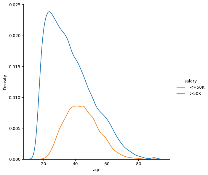
sns.displot(data=df, x="age", hue="salary", kind="kde", height=6, aspect=1)

<seaborn.axisgrid.FacetGrid at 0x7f17b8401950>

alt.Chart(df.sample(5000)).mark_point().encode(
    x="age",
    y='fnlwgt',
    color='salary',
    tooltip='education-num'
).facet(
    "sex"
).interactive()

Here I make two charts one is by using seaborn and the other one is by using altair, and also the second chart is interactive chart.As we can see from the charts, a large number of people get a salary of more than 50k when they are between 20 and 40 years old, but the number begins to decline after the age of 40

plt.figure(figsize=(12,5))
sns.countplot(data =df , x = 'workclass', hue = 'salary')
plt.show()

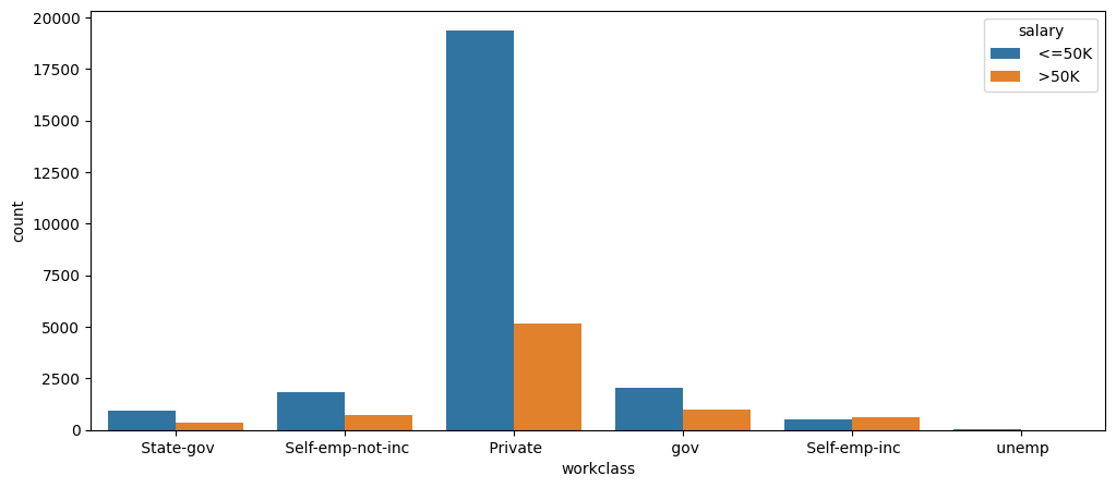
According to the bar graph, we can analyze that there are more people working in private enterprises, but from the proportion of count people, I think self-employees are more likely to get a salary of more than 50k

for i in df['native-country'] :
    if i != ' United-States':
        df['native-country'].replace([i] , 'Others' , inplace = True)
plt.pie(df['native-country'].value_counts() , labels = ['US' ,'Others'] , autopct = '%0.2f')
plt.show()

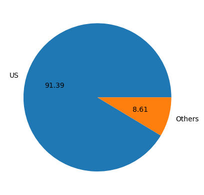
Here I classiy native-country columns to two variables in order to make a better pie. chart. From the pie chart, we can see that most of the data come from United States, So I think this data is not representative, we can ignore the impression of regions for a moment, we can consider all regions as the United States

encoder = LabelEncoder()
df["salary_num"] = df["salary"]
df['salary_num'] = encoder.fit_transform(df['salary_num'])
sns.histplot(df[df['salary_num'] ==0]['marital-status'])
sns.histplot(df[df['salary_num'] ==1]['marital-status'] , color='red')

<AxesSubplot:xlabel='marital-status', ylabel='Count'>

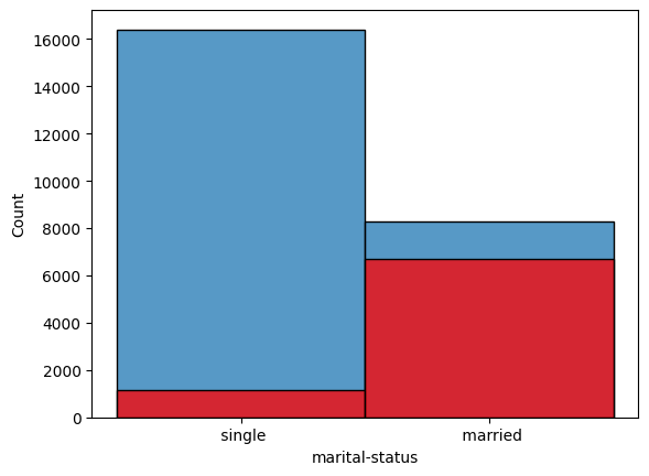
I use laberencoder to mark salary to 0 and 1, so it is easier for me to make the chart. And I make a new column salary_num here becasue I need to drop this column when I use train_test_split. From the Chart we can see that, most of married people earn more than 50k. I use seaborn to make this chart, because I think by using this method we can see more clear.

sns.kdeplot(data=df, x='hours-per-week', hue='salary')

<AxesSubplot:xlabel='hours-per-week', ylabel='Density'>

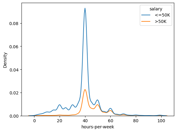
Because of laws, most of people work 40 hours a week, so this is real common.

plt.figure(figsize=(11,7))
sns.heatmap(df.corr(),annot=True)
plt.show()

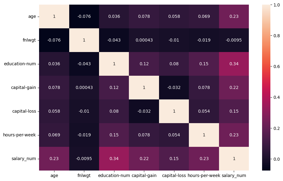
The heat map looks good.

Decison Tree Classifier#

encoder = LabelEncoder()
df = df.drop(["salary_num"],axis =1)
df['sex'] = encoder.fit_transform(df['sex'])
df['workclass'] = encoder.fit_transform(df["workclass"])
df["marital-status"] = encoder.fit_transform(df["marital-status"])
df["race"] = encoder.fit_transform(df["race"])
df["education"] = encoder.fit_transform(df["education"])
df["occupation"] = encoder.fit_transform(df["occupation"])
df["native-country"] = encoder.fit_transform(df["native-country"])
df["relationship"] = encoder.fit_transform(df["relationship"])

Here, we all know that we need to convert string values to integer values to divide the data and build trees. So here I use laberEncoder to convert my data. And I will post the web link in reference.

input_cols = [c for c in df.columns if c != "salary"]
X = df[input_cols]
y = df["salary"]
X_train,X_test,y_train,y_test = train_test_split(X,y,train_size=0.9,random_state=0)

This step is used to split the data, I want to set “salary” column to y and others to X. And I use 90% of the train_size

clf = DecisionTreeClassifier(max_leaf_nodes=30, max_depth= 20)
clf.fit(X_train,y_train)
fig = plt.figure(figsize=(20,10))
_=plot_tree(clf,
feature_names=clf.feature_names_in_,
class_names=clf.classes_,
filled=True)

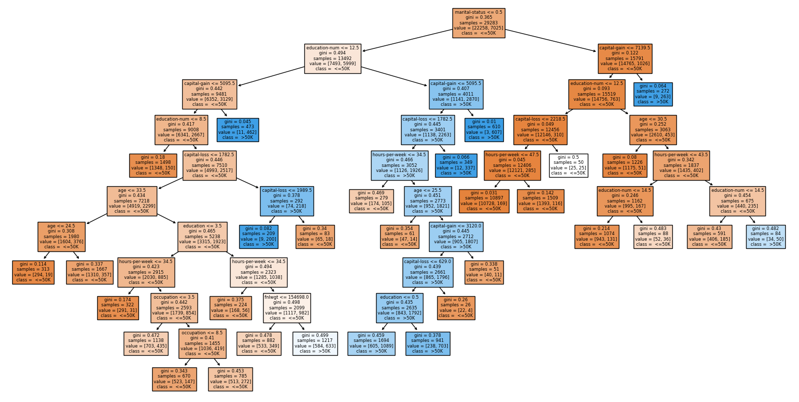
This step is used to build my decision tree. If there is a new person, we can go through this decision tree to classify his condition and finally get his salary whether it is above 50k or below 50k

pd.Series(clf.feature_importances_,index=clf.feature_names_in_).sort_values(ascending = True)

workclass         0.000000
relationship      0.000000
race              0.000000
sex               0.000000
native-country    0.000000
fnlwgt            0.003259
occupation        0.004738
education         0.013617
hours-per-week    0.027949
age               0.035311
capital-loss      0.056571
capital-gain      0.205799
education-num     0.221222
marital-status    0.431533
dtype: float64

This step is to rank feature importance.

print(clf.score(X_train,y_train))
print(clf.score(X_test,y_test))
accuracy = clf.score(X_test,y_test)*100
f"Accuracy on Test Data : {accuracy} %."

0.8570501656251067
0.8607867240319607

'Accuracy on Test Data : 86.07867240319607 %.'

Here I print train and test accuaracy by using f-string, and the result seems good.

Summary#

Either summarize what you did, or summarize the results. Maybe 3 sentences.

In my project, I first clean the data, and then I did the data visualization. Then I builed decision tree, after that I test the accuracy. According to the decision tree I made, if there is a new person, we can classify him according to his different conditions and eventually we can determine whether his salary will be higher than 50k.