Week 7 Wednesday#

Announcements#

I’m going to move my Wednesday office hours to my office RH 440J (same time: 1pm).
The next videos and video quizzes are posted. Due Monday of Week 8 (because Friday is a holiday this week).
Big topics left in the class: overfitting and decision trees/random forests.
Midterm: Tuesday of Week 9. On Wednesday of Week 9 (day before Thanksgiving) I’ll introduce the Course Project. (No Final Exam in Math 10.)

Including a categorical variable in our linear regression#

Here is some of the code from the last class. We used one-hot encoding to convert the “origin” column (which contains strings) into three separate numerical columns (containing only 0s and 1s, like a Boolean Series).

We haven’t performed the linear regression yet using these new columns.

import pandas as pd
import numpy as np

import altair as alt
import seaborn as sns

from sklearn.linear_model import LinearRegression
from sklearn.preprocessing import OneHotEncoder

df = sns.load_dataset("mpg").dropna(axis=0)

cols = ["horsepower", "weight", "model_year", "cylinders"]

reg = LinearRegression()

reg.fit(df[cols], df["mpg"])

LinearRegression()

In a Jupyter environment, please rerun this cell to show the HTML representation or trust the notebook.
On GitHub, the HTML representation is unable to render, please try loading this page with nbviewer.org.

pd.Series(reg.coef_, index=reg.feature_names_in_)

horsepower   -0.003615
weight       -0.006275
model_year    0.746632
cylinders    -0.127687
dtype: float64

encoder = OneHotEncoder()

encoder.fit(df[["origin"]])

OneHotEncoder()

new_cols = list(encoder.get_feature_names_out())

new_cols

['origin_europe', 'origin_japan', 'origin_usa']

df2 = df.copy()

df2[new_cols] = encoder.transform(df[["origin"]]).toarray()

df2.sample(5, random_state=12)

	mpg	cylinders	displacement	horsepower	weight	acceleration	model_year	origin	name	origin_europe	origin_japan	origin_usa
146	28.0	4	90.0	75.0	2125	14.5	74	usa	dodge colt	0.0	0.0	1.0
240	30.5	4	97.0	78.0	2190	14.1	77	europe	volkswagen dasher	1.0	0.0	0.0
82	23.0	4	120.0	97.0	2506	14.5	72	japan	toyouta corona mark ii (sw)	0.0	1.0	0.0
1	15.0	8	350.0	165.0	3693	11.5	70	usa	buick skylark 320	0.0	0.0	1.0
345	35.1	4	81.0	60.0	1760	16.1	81	japan	honda civic 1300	0.0	1.0	0.0

This is where the new (Wednesday) material begins. Let’s start with a reminder of what the one-hot encoding is doing. There are three total values in the “origin” column. We definitely can’t use this column “as is” for linear regression, because it contains strings. In theory we could replace the strings with numbers, like 0,1,2, but that would enforce an order on the categories, as well as the relative difference between the categories. Instead, at the cost of taking up more space, we make three new columns.

df["origin"]

       usa
       usa
       usa
       usa
       usa
        ...  
     usa
  europe
     usa
     usa
     usa
Name: origin, Length: 392, dtype: object

This particular NumPy array would be two-thirds zeros (why?). If there were more values, it would be even more dominated by zeros. For this reason, to be more memory-efficient, by default, scikit-learn saves the result as a special “sparse” object.

encoder.fit_transform(df[["origin"]])

<392x3 sparse matrix of type '<class 'numpy.float64'>'
	with 392 stored elements in Compressed Sparse Row format>

We can convert this to a normal NumPy array by using the toarray method.

encoder.fit_transform(df[["origin"]]).toarray()

array([[0., 0., 1.],
       [0., 0., 1.],
       [0., 0., 1.],
       ...,
       [0., 0., 1.],
       [0., 0., 1.],
       [0., 0., 1.]])

Here is a reminder of the last five values in the “origin” column.

df["origin"][-5:]

     usa
  europe
     usa
     usa
     usa
Name: origin, dtype: object

Here are the corresponding rows of the encoding. Notice how most of the 1 values correspond in the last column (corresponding to “usa”), and the other 1 value is in the first column (corresponding to “europe”. Be sure you understand how the 5 entries in the “origin” column correspond to this 5x3 NumPy array.

encoder.fit_transform(df[["origin"]]).toarray()[-5:]

array([[0., 0., 1.],
       [1., 0., 0.],
       [0., 0., 1.],
       [0., 0., 1.],
       [0., 0., 1.]])

df.columns

Index(['mpg', 'cylinders', 'displacement', 'horsepower', 'weight',
       'acceleration', 'model_year', 'origin', 'name'],
      dtype='object')

It wouldn’t make sense to use one-hot encoding on the “name” column, because almost every row has a unique name.

df.name[-5:]

  ford mustang gl
        vw pickup
    dodge rampage
      ford ranger
       chevy s-10
Name: name, dtype: object

len(df["name"].unique())

Let’s finally see how to perform linear regression using this newly encoded “origin” column. We specify that this linear regression object should not learn the intercept. (We’ll say more about why a little later in this notebook.)

reg2 = LinearRegression(fit_intercept=False)

We now fit this object using the 4 old columns and the 3 new columns.

reg2.fit(df2[cols+new_cols], df2["mpg"])

LinearRegression(fit_intercept=False)

Because we set fit_intercept=False, the intercept_ value is 0.

reg2.intercept_

0.0

More interesting are the seven coefficients.

reg2.coef_

array([-1.00027917e-02, -5.73669613e-03,  7.57614205e-01,  1.42568914e-01,
       -1.55580718e+01, -1.52649392e+01, -1.75931922e+01])

Here they are, grouped with the corresponding column names. Originally I was going to use index=cols+new_cols, but this approach, using index=reg2.feature_names_in_, is more robust.

pd.Series(reg2.coef_, index=reg2.feature_names_in_)

horsepower       -0.010003
weight           -0.005737
model_year        0.757614
cylinders         0.142569
origin_europe   -15.558072
origin_japan    -15.264939
origin_usa      -17.593192
dtype: float64

Finding those coefficients is difficult, but once we have the coefficients, scikit-learn is not doing anything fancy when it makes its predictions. Let’s try to mimic the prediction for a single data point.

df.loc[153]

mpg                       18.0
cylinders                    6
displacement             250.0
horsepower               105.0
weight                    3459
acceleration              16.0
model_year                  75
origin                     usa
name            chevrolet nova
Name: 153, dtype: object

With some rounding, the following is the computation made by scikit-learn. Look at these numbers and try to understand where they come from. For example, 105 is the “horsepower” value, and -0.01 is the corresponding coefficient found by reg2.

Notice also the -17.59 at the end. This corresponds to the origin_usa value. This ending will always be the same for every car with “origin” as “usa”. This -17.59 is not being multiplied by anything (or, if you prefer, it is being multiplied by 1), so it functions like an intercept, a custom intercept for the “usa” cars. This is the reason why we set fit_intercept=False when we created reg2. Another way to look at it, is if we wanted to add for example 13 as an intercept, we could just add 13 to the “origin_europe” value, to the “origin_japan” value, and to the “origin_usa” value; that would have the exact same effect.

105*-0.01+3459*-0.0057+0.757*75+0.142*6+-17.59

19.270699999999994

Let’s try to recover that number using reg2.predict. We can’t use the following because it is a pandas Series, and hence is one-dimensional.

df2.loc[153, cols+new_cols]

horsepower       105.0
weight            3459
model_year          75
cylinders            6
origin_europe      0.0
origin_japan       0.0
origin_usa         1.0
Name: 153, dtype: object

By replacing the integer 153 with the list [153], we get a pandas DataFrame with a single row.

df2.loc[[153], cols+new_cols]

	horsepower	weight	model_year	cylinders	origin_europe	origin_japan	origin_usa
153	105.0	3459	75	6	0.0	0.0	1.0

Now we can use reg2.predict. The resulting value isn’t exactly the same as above (19.19 instead of 19.27), but I think this distinction is just due to the rounding I did when typing out the coefficients.

reg2.predict(df2.loc[[153], cols+new_cols])

array([19.18976159])

Polynomial regression#

In linear regression, we find the linear function that best fits the data (“best” meaning it minimizes the Mean Squared Error, discussed more in this week’s videos).

In polynomial regression, we fix a degree d, and then find the polynomial function that best fits the data. We use the same LinearRegression class from scikit-learn, and if we use d=1, we will get the same results as linear regression.

Using polynomial regression with degree d=3, model “mpg” as a degree 3 polynomial of “horsepower”. Plot the corresponding predicted values.

I had intended to use PolynomialFeatures from scikit-learn.preprocessing, but because we were low on time, I used a more basic approach.

# There is a fancier approach using PolynomialFeatures
df.head(3)

	mpg	cylinders	displacement	horsepower	weight	acceleration	model_year	origin	name
0	18.0	8	307.0	130.0	3504	12.0	70	usa	chevrolet chevelle malibu
1	15.0	8	350.0	165.0	3693	11.5	70	usa	buick skylark 320
2	18.0	8	318.0	150.0	3436	11.0	70	usa	plymouth satellite

The main trick is to add columns to the DataFrame corresponding to powers of the “horsepower” column. Then we can perform linear regression. Phrased another way, if \(x_2 = x^2\), then finding a coefficient of \(x_2\) is the same as finding a coefficient of \(x^2\).

With a higher degree, you should use a for loop. I just typed these out by hand to keep things moving faster.

df["h2"] = df["horsepower"]**2

df["h3"] = df["horsepower"]**3

Notice how we have two new columns on the right. For example, the “h2” value of 16900 in the top row corresponds to 130**2.

df.head(3)

	mpg	cylinders	displacement	horsepower	weight	acceleration	model_year	origin	name	h2	h3
0	18.0	8	307.0	130.0	3504	12.0	70	usa	chevrolet chevelle malibu	16900.0	2197000.0
1	15.0	8	350.0	165.0	3693	11.5	70	usa	buick skylark 320	27225.0	4492125.0
2	18.0	8	318.0	150.0	3436	11.0	70	usa	plymouth satellite	22500.0	3375000.0

Let’s use Linear Regression with these columns (equivalently, we are using polynomial regression of degree 3 with the “horsepower” column).

It would be more robust to call these instead ["h1", "h2", "h3"] and to make the list using list comprehension. That is what you’re asked to do on Worksheet 12.

poly_cols = ["horsepower", "h2", "h3"]

reg3 = LinearRegression()

reg3.fit(df[poly_cols], df["mpg"])

LinearRegression()

We add the predicted value to the DataFrame.

df["poly_pred"] = reg3.predict(df[poly_cols])

Here we plot the predicted values. Take a moment to be impressed that linear regression is what produced this curve which is clearly not a straight line. Something that will be emphasized in Worksheet 12, is that as you use higher degrees for polynomial regression, the curves will eventually start to “overfit” the data. This notion of overfitting is arguably the most important topic in Machine Learning.

c = alt.Chart(df).mark_circle().encode(
    x="horsepower",
    y="mpg",
    color="origin"
)

c1 = alt.Chart(df).mark_line(color="black", size=3).encode(
    x="horsepower",
    y="poly_pred"
)

c+c1

Not related to polynomial regression directly, but I wanted to keep the following “starter” code present in the notebook. It shows an example of specifying a direct numerical value for y. The following could be considered the best “degree zero” polynomial for this data.

c = alt.Chart(df).mark_circle().encode(
    x="horsepower",
    y="mpg",
    color="origin"
)

c1 = alt.Chart(df).mark_line(color="black", size=3).encode(
    x="horsepower",
    y=alt.datum(df["mpg"].mean())
)

c+c1

Warning: Don’t misuse polynomial regression#

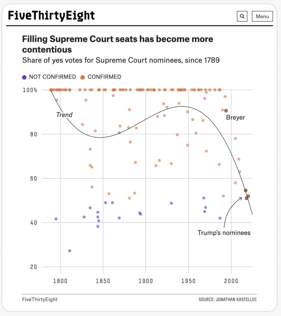
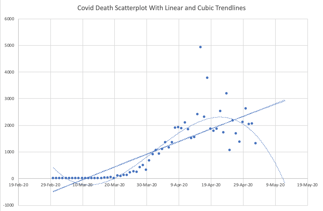
For some reason, unreasonable cubic models often get shared in the media. The cubic polynomial that “fits best” can be interesting to look at, but don’t expect it to provide accurate predictions in the future. (This is a symptom of overfitting, which is a key concept in Machine Learning that we will return to soon.)

In the following, from May 2020, if we trusted the linear fit, we would expect Covid deaths to grow without bound at a constant rate forever. If we trusted the cubic fit, we would expect Covid deaths to hit zero (and in fact to become negative) by mid-May.

Cubic fit to Covid data

The following is another example of a cubic fit. To my eyes, when I look at this data, I do not see anything resemblance to the shown cubic polynomial. That cubic polynomial is probably the “best” cubic polynomial for this data, but I do not think it is a reasonable model for this data (meaning I don’t think any cubic polynomial would model this data well).

Cubic fit to supreme court confirmation votes

UC Irvine Math 10, Fall 2022

Week 7 Wednesday

Contents

Week 7 Wednesday#

Announcements#

Including a categorical variable in our linear regression#

Polynomial regression#

Warning: Don’t misuse polynomial regression#